Hi guys, so this blog is about various attention mechanisms available, most popularly we are looking into Bahdanau and Luong variants. The problem we are facing right now is the context vector from the encoder last time step does not capture long term dependencies. Various authors has proposed a method of using a dynamic context vector for each decoder time step instead of a static context vector received from last encoder timestep. A encoder RNN gives us two things, one is the outputs of the encoder of all timesteps and the other is the hidden vector of the last timestep in each layer. In our old approaches, we took advantage of the latter output, we made use of the last timestep hidden vector as the initial state for the decoder, to establish a link between encoder and decoder. But we are not taking leverage of the encoder outputs from all timesteps. Authors told that lets allow each decoder timestep to look at all encoder outputs and focus its attention on the desired timestep instead of us forcing to it look at only last timestep hidden vector. Below is the old approach people followed before attention,
VOCAB_SIZE = 20
EMBEDDING_DIM = 64
HIDDEN_SIZE = 128
ATTENTION_SIZE = 128

class ReverseTaskV0(nn.Module):
    """
    This Architecture involves the usage of a Encoder - Decoder system connected by a context vector
    The encoder/decoder architecture is build using a vanilla RNN
    """
    def __init__(self):
        super().__init__()
        self.enc_embeddings = nn.Embedding(VOCAB_SIZE, EMBEDDING_DIM)
        self.encoder = nn.RNN(input_size=EMBEDDING_DIM, hidden_size=HIDDEN_SIZE, batch_first=True)

        self.dec_embeddings = nn.Embedding(VOCAB_SIZE, EMBEDDING_DIM)
        self.decoder = nn.RNN(input_size=EMBEDDING_DIM, hidden_size=HIDDEN_SIZE, batch_first=True)
        self.output_layer = nn.Linear(in_features=HIDDEN_SIZE, out_features=VOCAB_SIZE)

    def forward(self, enc_inputs, dec_inputs):
        """
        :param enc_inputs: (B, S) -> 32, 10
        :param dec_inputs: (B, S) -> 32, 10
        :return: logits -> (B, S, Vocab_size) -> 32, 10, 20
        """
        enc_emb = self.enc_embeddings(enc_inputs) #(B, S, emb_dim) -> 32, 10, 32
        enc_out, enc_hidden = self.encoder(enc_emb) #(B, S, H), (L, B, H) -> (32, 10, 16), (1, 32, 16)

        dec_emb = self.dec_embeddings(dec_inputs)#(B, S, emb_dim) -> 32, 10, 32
        dec_out, dec_hidden = self.decoder(dec_emb, enc_hidden) #(B, S, H), (L, B, H) -> (32, 10, 16), (1, 32, 16)
        logits = self.output_layer(dec_out) #B, S, V -> 32, 10, 20
        return logits
1. Bahdanau Additive Attention Implementation
In the implementation, at each decoder timestep the decoder receives a dynamically computed context vector using the encoder outputs. The way Bahdanau developed this context vector(ct) is given below :
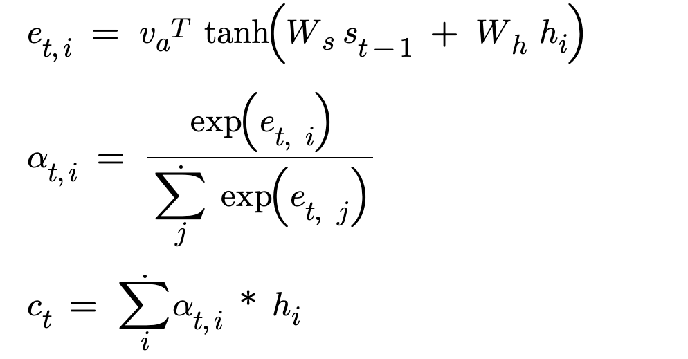
Lets get the variables straight, each decoder time step is t and each encoder output is traversed through ‘i’. We must find how similar is the previous decoder hidden vector with each encoder output. This similarity score is given by e_t,i for a ‘t’ decoder time step and ‘i’ encoder output. h_i is the encoder output at the ith timestep and s_t-1 is the previous decoder hidden vector.
- We take the encoder output and project it from encoder space to the attention space. W_h is a Linear layer of in_features equal to encoder hidden size and out_features is a attention size hyperparameter. W_h * h_i is famously called the encoder projection. We convert a vector of encoder hidden size to a vector of attention size.
- We take the previous decoder hidden vector and project it from decoder space to the attention space. W_s is a Linear layer of in_features equal to decoder hidden size and out_features equal to attention size W_s * s_t-1 is famously called the decoder projection. We convert a vector of decoder hidden size to a vector of attention size.
- We add both the projections and that is why implementation has its name additive attention. This added projections has both the information about the encoder state and the decoder previous state.
- We need a similarity score, we compute the dot product between the added projection vector and the attention vector v_a of attention size. This similarity score is e_t,i
- We convert these attention scores to attention weights by computing softmax over the raw values to get probabilities
- These attention weights are used to scale the encoder outputs or more simply we use the attention weights to add weightage to the encoder outputs and build the dynamic context vector.
Lets look at the code and develop the entire architecture.
class ReverseTaskV6(nn.Module):
    """
    This architecture implements Bahdanau Additive attention implementation
    """
    def __init__(self):
        super().__init__()
        self.enc_embeddings = nn.Embedding(VOCAB_SIZE, EMBEDDING_DIM)
        self.encoder = nn.GRU(input_size=EMBEDDING_DIM, hidden_size=HIDDEN_SIZE, batch_first=True)

        self.dec_embeddings = nn.Embedding(VOCAB_SIZE, EMBEDDING_DIM)
        self.decoder = nn.GRU(input_size=EMBEDDING_DIM + HIDDEN_SIZE, hidden_size=HIDDEN_SIZE, batch_first=True)

        self.W_h = nn.Linear(HIDDEN_SIZE, ATTENTION_SIZE) #for encoder projection where encoder output is h_i
        self.W_s = nn.Linear(HIDDEN_SIZE, ATTENTION_SIZE) #for decoder projection where prev decoder hidden state is s_t-1
        self.v = nn.Linear(ATTENTION_SIZE, 1, bias=False) #turns the vector to a score

        self.output_layer = nn.Linear(HIDDEN_SIZE, VOCAB_SIZE)

    def forward(self, enc_inputs, dec_inputs):
        #enc_inputs : (B, S), dec_inputs : (B, S)
        enc_emb = self.enc_embeddings(enc_inputs) #B, S, E
        enc_out, enc_hidden = self.encoder(enc_emb) # (B, S, H), (1, B, H)

        dec_timesteps = dec_inputs.shape[1]
        prev_hidden = enc_hidden  #s_t-1 (1, B, H)
        outputs = []
        for t in range(dec_timesteps):
            #For every timestep : build the context vector ct using enc_outputs
            enc_proj = self.W_h(enc_out) #B, S, A
            dec_proj = self.W_s(prev_hidden)#1, B, A
            dec_proj = dec_proj.squeeze(dim=0).unsqueeze(dim=1) # 1, B, A -> B, A -> B, 1, A

            add_projections = torch.tanh(enc_proj + dec_proj) #B, S, A + B, 1, A => after broadcasting on dim=1 -> B, S, A
            # add_proj is the vector of combined info from prev hidden and each enc output. Each timestep has  attention vector
            scores = self.v(add_projections).squeeze(dim=-1) #B, S, A => B, S,1 => B, S-> This turns attention vector to attention score

            probs = torch.softmax(scores, dim=1) #converts attention score to attention weights #B, S
            context_vector = torch.bmm(probs.unsqueeze(dim=1), enc_out) #bmm of (B, 1, S) @ (B, S, H) -> B, 1, H
            # -> take the attention score of each timestep and turn it a vector of timesteps.
            # Element of this vector is multiplied with hidden vector at each time step(scaling the hidden vector).
            # Scaled hidden vector for all time steps is blended together into a single vector by adding its elements across hidden size dimension

            #Build the embedding vector
            emb_vector = self.dec_embeddings(dec_inputs[:, t]).unsqueeze(dim=1) #B, 1, E

            #Prepare input for decoder step
            s_t = torch.cat([emb_vector, context_vector],dim=2)#(B, 1, E) + (B, 1 , H) = B, 1, E+H
            dec_out_t , dec_hidden = self.decoder(s_t, prev_hidden) #(B, 1, H),( 1, B, H)

            logits = self.output_layer(dec_out_t) #B, 1, V
            outputs.append(logits)
            prev_hidden = dec_hidden

        return torch.cat(outputs, dim=1)
Let me just explain the decoder time step loop and rest of the others are self-explanatory. For every time step, we build the context vector using the above described process. For the input at the time step ‘t’, build a embedding vector. The concatenated(it’s not added) result is the input for the decoder time step instead of giving only the embedding vector which was originally did. We concatenate the embedding information and context information is to preserve the meaning. Also now the input of the decoder has more information to generate a good token.
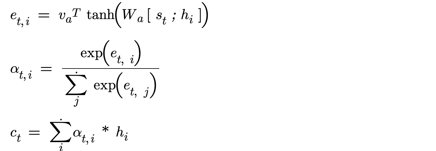
2. Bahdanau Concatenative Attention Implementation
In the paper Neural Machine Translation by Bahdanau, he has concatenated the encoder outputs and decoder previous hidden vector.

As we can see clearly, from the above set of formulas that way of calculating similarity score(e_t,i) changed and rest of the process remains the same. In the calculation of similarity score, the author has concatenated the encoder outputs and decoder hidden vector, due to this the resultant vector will of encoder hidden size and decoder hidden size. During addition, it works element wise and there is no change in dimension. More conceptually during addition the two information is mixed together. During concatenation the two information is combined/appended together to preserve the meaning, thus the size of vector increases.
As for our concatenation case, the size of the concatenated vector is encoder hidden size and decoder hidden size. The vector needs to be projected to the attention space using W_a which is a linear layer of in_features equal to encoder hidden size and decoder hidden size, out_Features is equal to attention size. This projected vector will later be multiplied with attention vector to get a similarity score.
Bahdanau in his paper has exhibited this concatenation appraoch and reasearchers often using a mathematically equivalent additive approach explained before as the attention mechanism. Both the additive and concatenative approach are mathematically equivalent and additive approach is relatively easier to implement. Honestly, In my opinion concatenative is simpler, there is only one weight matrix and less parameters but who cares folks.Let’s move to next type.
3. Luong Dot Attention Implementation
Luong has provided his own set of approaches in his paper Effective Approaches to Attention-based Neural Machine Translation. For Luong dot attention, he has established the following equations,
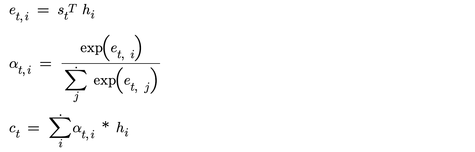
As we can see, equations are much simpler. The similarity score e_t,i we are trying to find between the encoder outputs and the decoder hidden state, is just a similarity check. In order to compute similarity between 2 vectors,
Why apply non-linearity(using tanh)?
Why project vectors from their space to attention space?
Why use a redundant attention vector (v_a)?
Luong asked all these questions and implemented a simple dot product between encoder outputs and decoder hidden state, If you guys are not aware dot product is computed on 2 vectors and it shows how similar two vectors are. Dot product also returns a single score which in our case will be called as attention score. This made all the calculations much easier. Now let’s implement in torch!!
class ReverseTaskV8(nn.Module):
    """
    This architecture implements Luong dot attention implementation
    """
    def __init__(self):
        super().__init__()
        self.enc_embeddings = nn.Embedding(VOCAB_SIZE, EMBEDDING_DIM)
        self.encoder = nn.GRU(input_size=EMBEDDING_DIM, hidden_size=HIDDEN_SIZE, batch_first=True)

        self.dec_embeddings = nn.Embedding(VOCAB_SIZE, EMBEDDING_DIM)
        self.decoder = nn.GRU(input_size=EMBEDDING_DIM, hidden_size=HIDDEN_SIZE, batch_first=True)

        self.output_layer = nn.Linear(2*HIDDEN_SIZE, VOCAB_SIZE)

    def forward(self, enc_inputs, dec_inputs):
        #enc_inputs : (B, S), dec_inputs : (B, S)
        enc_emb = self.enc_embeddings(enc_inputs) #B, S, E
        enc_out, enc_hidden = self.encoder(enc_emb) # (B, S, H), (1, B, H)

        dec_timesteps = dec_inputs.shape[1]
        prev_hidden = enc_hidden  #s_t-1 (1, B, H_d)

        outputs = []
        for t in range(dec_timesteps):
            #Build the embedding vector
            emb_vector = self.dec_embeddings(dec_inputs[:, t]).unsqueeze(dim=1) #B, 1, E

            dec_out , dec_hidden = self.decoder(emb_vector, prev_hidden) #(B, 1, H),( 1, B, H)

            #Build the context vector ct using enc_outputs
            s_t = dec_hidden[-1] #B, H #to fetch the hidden of last layer

            scores = torch.bmm(enc_out, s_t.unsqueeze(dim=2)) #B, S, H @ B, H, 1 => B, S, 1

            probs = torch.softmax(scores, dim=1) #converts attention score to attention weights #B, S, 1

            context_vector = torch.bmm(probs.transpose(1, 2), enc_out) #bmm of transpose((B, S, 1)) @ (B, S, H) -> B, 1, H
            # -> take the attention score of each timestep and turn it a vector of timesteps.
            # Element of this vector is multiplied with hidden vector at each time step(scaling the hidden vector).
            # Scaled hidden vector for all time steps is blended together into a single vector by adding its elements across hidden size dimension

            logits = self.output_layer(torch.cat([dec_out, context_vector], dim=2)) #B, 1, 2H -> B, 1, V
            outputs.append(logits)
            prev_hidden = dec_hidden

        return torch.cat(outputs, dim=1)
You might be confused, why we are building the embedding vector first instead of context vector, like we did in Bahdanau. Luong suggested that using the current timestep’s hidden state in the calculation of attention scores, is much more reasonable and accurate that using previous state. We first do the decoder pass, using the embedding vector and previous hidden. We fetch the hidden state and store in s_t (you can also verify in the equations that we have used s_t instead of s_t-1). We compute similarity and store it in attention scores. We use batch matrix multiplication which is a combination of multiple matrix multiplication, and each matrix multiplication is a combination of dot products. We are ultimately doing dot products but for batches of data and for all encoder timesteps using a single operation. Once we have build the context vector, we concatenate the context vector and decoder result for the output layer to provided logits for different tokens in vocabulary.(Hope you are already familiar with output layer concept)
4. Luong General Attention Implementation
This implementation is to fix the drawbacks/limitations of previous approach. In the previous approach, we did dot product between encoder outputs and decoder hidden state. Dot products only work when the dimensions of the two vectors match. For example, in our case, the encoder hidden size must match the decoder hidden size. If the dimensions doesn’t match then dot product fails. Also we cannot always guarantee that the hidden sizes will match or our architecture may/may not need same/different hidden sizes. For same hidden sizes, Luong dot attention is the best approach and for different hidden size, Luong General attention is the best approach.
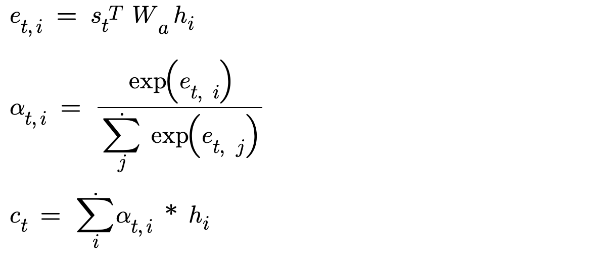
As you can see in the figure, we take the encoder outputs(h_i) and project it to decoder space, using a Linear layer. This layer has in_features of encoder hidden size and out_features of decoder hidden size. Now, our problem is solved. Now matter, any dimensional vector we have in encoder outputs, we can compute similarity for it.
class ReverseTaskV7(nn.Module):
    """
    This architecture implements Luong general attention implementation
    """
    def __init__(self):
        super().__init__()
        self.enc_embeddings = nn.Embedding(VOCAB_SIZE, EMBEDDING_DIM)
        self.encoder = nn.GRU(input_size=EMBEDDING_DIM, hidden_size=HIDDEN_SIZE, batch_first=True)

        self.dec_embeddings = nn.Embedding(VOCAB_SIZE, EMBEDDING_DIM)
        self.decoder = nn.GRU(input_size=EMBEDDING_DIM, hidden_size=HIDDEN_SIZE, batch_first=True)

        self.W = nn.Linear(HIDDEN_SIZE, HIDDEN_SIZE) #for projecting the vector from encoder space to decoder space

        self.output_layer = nn.Linear(2*HIDDEN_SIZE, VOCAB_SIZE)

    def forward(self, enc_inputs, dec_inputs):
        #enc_inputs : (B, S), dec_inputs : (B, S)
        enc_emb = self.enc_embeddings(enc_inputs) #B, S, E
        enc_out, enc_hidden = self.encoder(enc_emb) # (B, S, H), (1, B, H)

        dec_timesteps = dec_inputs.shape[1]
        prev_hidden = enc_hidden  #s_t-1 (1, B, H_d)

        enc_proj = self.W(enc_out) # => (B, S, H_e) -> (B, S, H_d)

        outputs = []
        for t in range(dec_timesteps):
            #Build the embedding vector
            emb_vector = self.dec_embeddings(dec_inputs[:, t]).unsqueeze(dim=1) #B, 1, E

            dec_out , dec_hidden = self.decoder(emb_vector, prev_hidden) #(B, 1, H),( 1, B, H)

            #Build the context vector ct using enc_outputs
            s_t = dec_hidden[-1] #B, H

            scores = torch.bmm(enc_proj, s_t.unsqueeze(dim=2)) #B, S, H @ B, H, 1 => B, S, 1

            probs = torch.softmax(scores, dim=1) #converts attention score to attention weights #B, S, 1

            context_vector = torch.bmm(probs.transpose(1, 2), enc_out) #bmm of (B, S, 1) @ (B, S, H) -> B, 1, H
            # -> take the attention score of each timestep and turn it a vector of timesteps.
            # Element of this vector is multiplied with hidden vector at each time step(scaling the hidden vector).
            # Scaled hidden vector for all time steps is blended together into a single vector by adding its elements across hidden size dimension

            logits = self.output_layer(torch.cat([dec_out, context_vector], dim=2)) #B, 1, 2H -> B, 1, V
            outputs.append(logits)
            prev_hidden = dec_hidden

        return torch.cat(outputs, dim=1)
5. Luong Concat Attention Implementation
This approach is very similar to Bahdanua concatenative attention and the single difference is Luong uses current hidden state and Bahdanu used previous hidden state.
That’s it guys. Hope you had a nice walkthrough on all the fancy attention mechanisms we have.