Abstract
Building a character level language model that learns patterns in data with next token prediction task. Used Tinyshakespeare text of 1MB from karpathy and build a 12M LM using a decoder-only transformer model.
Transformer Architecture
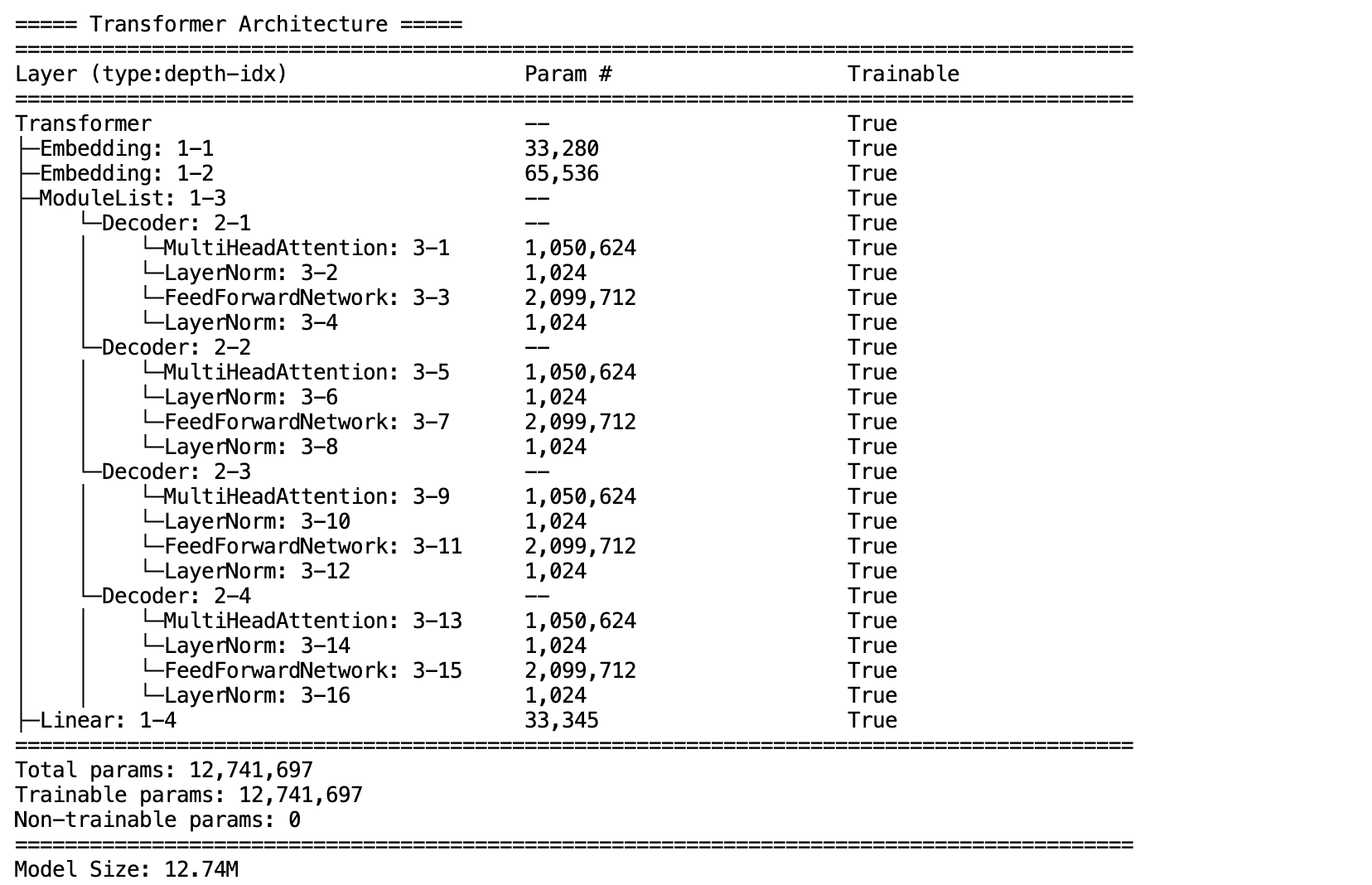
The architecture is fairly simple, it starts with an token embeddings, positional embeddings, a decoder block and output layer. In the decoder block, it has Multihead Attention, Layernorm and MLP (classical fully connected layers separated by activation non-linear functions).
Let’s take a single sentence as input. The first step is tokenization, where the sentence is broken down into smaller units called tokens. In a character-level language model, each character becomes a token. Since machine learning models work with numbers rather than text, each token is mapped to a unique integer known as a token ID.
These token IDs are then passed through an embedding layer, which learns a dense vector representation of size d_model for each token. The embedding captures semantic and syntactic information about the token. However, embeddings alone do not contain any information about the position of tokens in the sequence. Without positional information, the model would treat the input as a bag of tokens and would not know that, for example, “t” comes before “h” in the word “the”.
To address this, each position in the sequence is assigned a position ID (from 0 to sequence length − 1). A positional embedding is learned for each position, and this positional representation is added to the token embedding. The resulting vector contains information about both the token’s identity and its position in the sequence. At this stage, each token representation only contains information about itself and not about other tokens in the sequence.
The token representations are then passed through a stack of decoder blocks. Each decoder block consists of Masked Multi-Head Attention (MHA), Layer Normalization, and a Feed-Forward Network (FFN), along with residual (skip) connections.
In the attention layer, tokens interact with one another and learn contextual relationships. This transforms the token representations from self-aware representations into context-aware representations. Layer Normalization stabilizes training by normalizing each token’s activation vector so that its values have approximately zero mean and unit variance. The Feed-Forward Network then processes each token independently. In the original Transformer architecture described in the Attention Is All You Need paper, the FFN expands the representation from d_model to 4 × d_model and then projects it back to d_model.
Residual (skip) connections are introduced to make optimization easier. Instead of forcing a sub-layer to learn an entirely new representation from scratch, the sub-layer learns a modification to the existing representation. Mathematically, the output of a sub-layer is added to its input. If the sub-layer learns only a small adjustment, the original information is largely preserved. If the learned transformation is significant, the representation is modified accordingly. This helps maintain information flow and improves gradient propagation during training.
After passing through all decoder blocks, the final token representations are projected into the vocabulary space using an output linear layer. Dot product of each final token representation with vocabulary vectors gives a similarity score called logits. This produces a vector of logits for each token position, where each logit represents the model’s score for a possible next token in the vocabulary. Applying a softmax converts these logits into probabilities, and the next token is selected based on the chosen decoding strategy, such as greedy decoding.
Multi-Head Attention
Among all the components of the decoder, the attention mechanism is one of the most important. We start with the token representations and learn three different projections from them: Queries (Q), Keys (K), and Values (V). Instead of using a single attention head for all computations, the model employs multiple attention heads, allowing each head to learn its own set of queries, keys, and values from the input features (d_model). This gives different heads the flexibility to capture different types of relationships and patterns in the data.
Attention works by computing the similarity between queries and keys using a dot product (matrix multiplication). These similarity scores indicate how relevant one token is to another. The scores are then passed through a softmax function to obtain attention weights (probabilities). These weights are used to compute a weighted sum of the value vectors, producing a context-aware representation of each token.
A practical interpretation is that queries represent what a token is looking for, keys represent what a token offers, and values contain the actual information that can be retrieved.
During training, it was observed that the raw dot-product attention scores can have high variance, especially when the dimensionality of the key vectors is large. Large variance can cause the softmax function to become overly peaked, producing near one-hot distributions and leading to unstable gradients. To address this, the attention scores are scaled by dividing them by (\sqrt{d_k}), where (d_k) is the dimension of the key vectors.
Finally, in the decoder’s self-attention layer, a causal mask is applied to prevent tokens from attending to future tokens. This ensures that each token can only use information from previous tokens and itself, preventing the model from “cheating” by looking ahead when making predictions.
Training Character Language Model.
I used the Tiny Shakespeare dataset, which contains approximately 1 MB of text, and constructed training sequences of length 128. The first step was tokenizing the dataset at the character level, resulting in a vocabulary of 65 unique characters.
The model configuration is as follows:
- d_model = 512
- Number of decoder layers = 4
- Number of attention heads = 8
- Learning rate = 1e-3
- Batch size = 32
- Number of epochs = 10
With these settings, the character-level language model contains approximately 12 million trainable parameters and is trained to predict the next token given all preceding tokens in the sequence.
The training pipeline follows a standard deep learning workflow. First, the tokenized data is converted into tensors, wrapped in a TensorDataset, and loaded using a DataLoader. A random generator seed is used to ensure reproducibility. The model is then instantiated and moved to the target device (CPU or GPU), along with the input tensors.
To better understand the architecture, I implemented a helper function to inspect the number of trainable parameters in the model. Tools such as torchsummary or torchinfo can also be used to visualize the Transformer architecture and tensor shapes throughout the network.
The model outputs logits, which represent unnormalized scores over the vocabulary for each token position. Since the task is next-token prediction, it is formulated as a multi-class classification problem where the target is the true next token. Therefore, the appropriate loss function is Cross-Entropy Loss. For optimization, I used the Adam optimizer.
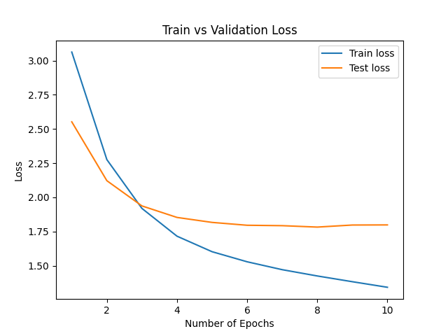
During training, I monitored the validation loss and checkpointed the model weights whenever a new best validation loss was achieved. The best validation loss obtained was approximately 1.79.
To evaluate the learning behavior, I plotted both the training and validation loss curves. The model learns effectively during the initial epochs; however, after approximately the fifth epoch, the validation loss begins to increase while the training loss continues to decrease. This divergence is a classic indicator of overfitting, where the model starts memorizing patterns specific to the training data rather than learning features that generalize well to unseen data. Given that the model contains around 12 million parameters while the dataset is only about 1 MB in size, the model capacity is relatively large for the amount of available training data, making overfitting expected.

Training Setup
The model was trained on a GPU-enabled remote machine accessed via SSH. The environment was configured using Docker, where I created a container with GPU access and configured it to remain running until explicitly stopped. Inside the container, I created a dedicated Conda environment, installed all required dependencies, and registered an IPython kernel to enable development and experimentation through Jupyter notebooks.
The machine is equipped with two NVIDIA RTX A6000 GPUs. However, given that the Transformer model contains approximately 12 million parameters, a single GPU provides more than sufficient computational resources for training. The available hardware offers ample memory and compute capacity, resulting in smooth training and experimentation without resource constraints.
Observations / Ablation study
I have experimented with a few scenarios in my model and observed how the validation loss behaves in each case.
1. Weight tying experiment
My first experiment was tying the weights of the embedding layer and the output layer to see if it improves the model. After weight tying, the first epoch training loss was around 21.76, whereas in the untied setup it was around 2.53.
I found that the embedding layer was initialized with a standard deviation of 1 (N(0, 1)), while the output linear layer was initialized with a standard deviation of 0.02.
Untied: token_embeddings.std() = 0.9994, output_layer.std() = 0.0255, train loss (1st epoch) = 2.53 Tied: token_embeddings.std() = 0.9994, output_layer.std() = 0.9994 (after tying, ~40× larger), train loss (1st epoch) = 21.78 The logits become very large, leading to a high initial loss. The expected random baseline loss is −log(1/65) ≈ 4.17.
To fix this, I initialized the embedding weights as:
nn.init.normal_(
    self.token_embeddings.weight,
    mean=0.0,
    std=0.02
)
After this fix, the model became stable. The untied setup gave a first epoch training loss of 3.06 and a best validation loss of 1.79. After fixing initialization, I applied weight tying again. Train Loss: 3.43 and Best Val Loss: 1.79 Verdict : Weight tying did not provide significant improvement.
Fixing my system, my train loss after first epoch : Train Loss : 3.06 and best val loss is 1.79 Secondly tie weights : Train Loss : 3.43, best val loss = 1.79
Verdict : it didn’t give big improvements
2. Pre-Norm vs Post-Norm
Pre-Norm Train loss: 3.06 → 1.28 Test loss: 2.55 → 1.83 Clear learning and Stable convergence
Post-Norm Train loss: ~3.35 → 3.31 (almost no change) Test loss: ~3.34 (flat) No learning and Training essentially stalled
In Pre-Norm, gradients flow smoothly through identity path, deep stacks are getting trained and with the help of gradients, optimizer updates and loss decreases as it learns. y=x+F(LN(x)) The residual connection is supposed to create a direct gradient highway and it keeps deep networks trainable.
In Post-Norm, every block output is normalized, residual signal is repeatedly rescaled and there is no identity path no more, gradients become harder to propagate backward, almost no gradients, no optimizer updates and loss remains the same. No learning in the setup. y=LN(x+F(x)) The residual connection is inside the layernorm and no direct path, input is not preserved. Repeated normalization and scaling across deep layers makes it harder to train deep neural networks since the identity is lost within layernorm.
3. Residual connection
With Residual connections Train loss: 3.06 → 1.28 Test loss: 2.55 → 1.83
There is clear learning and Stable convergence. Identity signal is always preserved, each layer only learns a correction and gradient has a direct shortcut path
Without Residual connections Train loss: ~3.35 → 3.31 (almost no change) Test loss: ~3.33 (flat)
Information gets overwritten at every layer and gradients must pass through many nonlinear transformations There is no direct path from input → output
Removing residual connections significantly degrades optimization stability and prevents deep layers from learning useful transformations. Residual connections act as an identity path that ensures stable gradient flow and allows each layer to learn incremental refinements rather than full transformations.
4. Dropout
Adding a dropout of 0.1 to the sublayers (attention and FFN) gave interesting results. In my baseline setup it converged in epoch 5 and later it starts to overfit. In dropout setup, Train loss decreases slightly slower and Best test loss reached around epoch 7–8. So Dropout improved generalization and reduced overfitting, but did not significantly change the final best achievable loss.
Dropout adds noise during training by randomly disabling neurons and prevents memorization. So harder to fit training data perfectly. The val loss is more smoother.