Hello guys, so I have been working on developing a Sequence-2-Sequence Architecture for the Neural Machine Translation Task. The idea is we have a encoder to process the source sentence. Each word in source sentence counts as a time step, at each time step encoder see the word at that time step and hidden vector( compressed representation of memory )from previous time step. At the final time step of the encoder it produces a hidden vector, this hidden vector is a summarized version of the source sentence. It is called the context vector.

Using this context vector, we pass it to the decoder model along with the previous target word in target sentence. Instead of starting the RNN from a randomly initialized vector like we did for encoder, we use the context vector for the decoder hence the name decoder.

In this blog, our main focus is on gradients tracking. First lets check out various problems we face with respect to gradients and then secondly we will check out the techniques that is very useful for us to analyze how gradients flow in our network .

Problems in Gradients:

1. Vanishing Gradients
2. Exploding Gradients

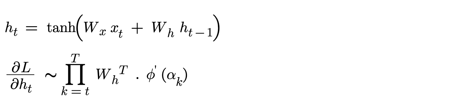
The two equations in the above figure is very important in order to understand how gradients vanish/explode. The first equation is computation of hidden state using input at that time step and previous hidden state. The second equation is gradient of hidden state with respect to loss. This gradient value can vanish / explode. As you look carefully in the second equation given a time step, the gradient of hidden vector is repeated multiplication of Weight matrices W_h. Let’s check out what vanishing and exploding gradients are.

Vanishing Gradients

During Backpropagation through time, gradients flow back in the network and get repeatedly multiplied by same weight matrix for each time step. Due to this gradients gets smaller and smaller as they go back to the leaf tensor. Typically gradients of value 1e-4 or less than it are considered vanishing gradients, it’s so tiny that it almost doesn’t contribute in optimizer step (gradients update). The change is very small. Let’s imagine we are passing a signal through 50 layers, each layer reduces it by 0.9, then after 50 steps, final signal is 0.9 ^ 50 ≈ 0.005. If you connect this with our equation we can find that gradients shrink exponentially. That is the problem we are facing, for long sequences there are more timesteps and if our weight matrices values are btw 0 to 1 then using this when the gradient of the hidden vector is computed then it’s values are almost zero.

Exploding Gradients

Similarly, During backpropagation through time, some gradients get larger as they propagate back through the network. This is also due to repeated multiplication of weight matrices but here the gradients explode exponentially. When a gradient value is 50, 100 or more, the gradients are exploding gradients. This is the range for us to say that training is not stable and not healthy. During exploding gradients, even loss turns NAN. Let’s once again imagine we are passing a signal through 50 layers, each layer increases it by 1.1 (just 1.1), then after 50 steps, final signal is 1.1 ^ 50 ≈ 117. Once again this is all due to weight matrices amplifying effect.

Linear Algebra Intuition :

This part is purely linear algebra, if you have a basic understanding in that field kindly proceed else skip this section. As Backpropagation happens, the derivative of hidden vector/state w.r.t to loss involves repeated multiplication of recurrent weight matrices. So the gradient vector is multiplied by W matrix many times as it propagates backward through timesteps. From linear algebra, We know that given a vector(h_t) and apply a transformation(W), such that if the transformation stretches space/collapses space and providing a scaled version (scale up/down) of the same vector. The value by which its scaled is eigen value.

v W = lambda v

Here lambda is the eigen value and v is our hidden vector. Eigenvalues tells us how a matrix/transformation scales a vector when we multiply by it. If a matrix’s eigen vector’s eigen values(lambda) is greater than 1, then hidden vector’s gradients explode. If the lambda is lesser than 1 then gradients vanish. Repeated multiplication of weight matrix means Repeated multiplication of eigen value to the same vector. This explodes/shrinks gradients exponentially.

Once solution is that weight matrix need to be orthogonal [ rotation transformation ], As they result in eigen value of 1 avoiding this problem completely.

Techniques to Track gradients.

Parameter information

This technique helps us understand the structure and capacity of the model before debugging training issues. By inspecting the total number of parameters, how many are trainable, and how they are distributed across layers, we get a clear picture of model complexity and potential bottlenecks. For example, if most parameters are concentrated in a specific layer, that layer may dominate learning. Similarly, a mismatch between expected and actual parameter counts can reveal architectural bugs. In short, this step answers: “What exactly are we training?” before asking “Why is it failing?”

def log_parameters_information(model):
    """
    Utility function to Bookkeep the parameters per layer, Total model parameters, Trainable and Non-Trainable Parameters
    """

    total_params = sum(p.numel() for p in model.parameters())
    print(f"Total params : {total_params}")

    trainable_params = sum(p.numel() for p in model.parameters() if p.requires_grad)
    print(f"Trainable params : {trainable_params}")
    print(f"Non Trainable params : {total_params - trainable_params }")

    print(f"Shape of parameters per layer")
    for name, param in model.named_parameters():
        print(name, param.shape)

    print(f"Count of parameters per layer")
    for name, param in model.named_parameters():
        print(name, param.numel())
        
#-------------------------- Log Parameters information  -----------------------------------

log_parameters_information(model)

This function takes the model and helps you print all the intricate details in it which are necessary for understanding our model architecture. Be cautions as for big architectures this might flood your logs.

Gradient Norms

Gradient norm represents the overall magnitude of the learning signal flowing through the network during backpropagation. Instead of looking at individual gradients, we compress all parameter gradients into a single scalar using the L2 norm, which tells us whether learning is happening effectively. If the norm is extremely small, updates become negligible (vanishing gradients), and if it is extremely large, updates become unstable (exploding gradients). Monitoring this value per batch gives a quick health check of training dynamics, helping us detect instability early.

Vanishing gradients - Gradient norms become very close to 0

Example: Total gradient norm: 0.000002 → 0.0000003 → 0.00000001

Exploding gradients - Gradient norms become extremely large

Example: Total gradient norm: 150 → 820 → 5000

loss.backward()

#-------------------------- Track Gradient Norm numerically per batch -----------------------------
total_norm = 0
for name, param in model.named_parameters():
    if param.grad is not None:
        grad_norm = param.grad.data.norm(2)
        total_norm += grad_norm.item() ** 2

total_norm = total_norm ** 0.5
print(f"Total gradient norm: {total_norm:.6f}")

optimizer.step()

Every parameter has a gradient, All the gradients together form one big vector and that is vector of gradients. If we calculate L2 norm(square each value of a vector and take a square root of all squares) then its gradient norm. Gradient norms close to zero means the gradients are vanishing, Gradient norms greater than 100 means the gradients are exploding. Gradient norms of 0.1 to 10 mean the training is stable and its healthy. Model is learning as well. This gradient norm code snippet is per batch and if you want per epoch level, use the next one.

Gradient Norms Visualization

While raw gradient norm values are useful, plotting them over training iterations reveals trends and patterns that are otherwise hard to notice. A stable training process typically shows smooth and bounded gradient norms, whereas erratic spikes indicate instability and collapsing values indicate vanishing gradients. This visualization helps us understand whether issues are persistent or temporary, and whether training is converging, diverging, or oscillating. Essentially, it answers: “How is the learning signal evolving over time?”

grad_norms = []

#-----Inside training loop ----

loss.backward()

total_norm = 0
for param in model.parameters():
    if param.grad is not None:
        total_norm += param.grad.data.norm(2).item() ** 2

total_norm = total_norm ** 0.5
grad_norms.append(total_norm)

optimizer.step()

#------------------   Track Gradient Norm visually across batches for a single epoch  -----------------------

plt.plot(grad_norms)
plt.title("Gradient Norm During Training")
plt.xlabel("Iterations")
plt.ylabel("Gradient Norm")
plt.show()

You can use this code to understand the scale of gradients and how its evolving/declining/juggling around iterations of training.

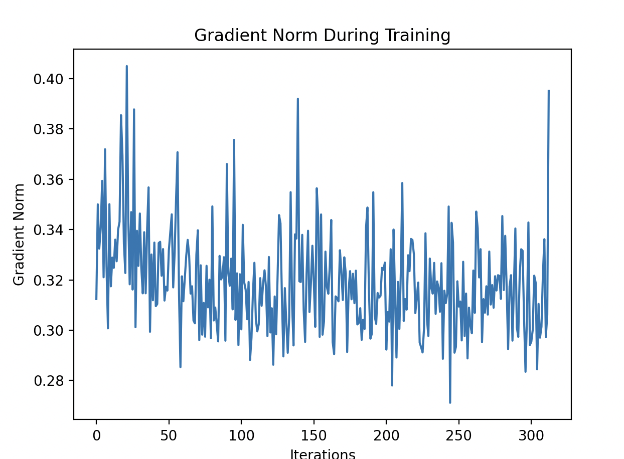
From the picture, we can observe that are gradients are not varying drastically by scale and the range looks reasonable here.

Layer-wise gradients

Instead of treating the model as a single unit, this technique breaks down gradients layer by layer to identify where learning is failing. Different parts of the network may behave very differently—some layers may receive strong gradients while others receive almost none. This is especially important in deep or sequential models like encoder-decoder architectures, where earlier layers (like the encoder) often suffer from vanishing gradients. By inspecting layer-wise gradient magnitudes, we can pinpoint exactly which part of the network is not learning and take targeted action.

loss.backward()
#------------ Inspecting layer wise gradients to identify which layer vanishes or explodes --------------

for name, param in model.named_parameters():
    if param.grad is not None:
        print(name, param.grad.abs().mean().item())

optimizer.step()

This tells you which layer vanishes.

Example:

encoder.weight grad = 1e-7

decoder.weight grad = 0.02

Encoder gradients vanish.

Also, always check gradients before you call optimizer.zero_grad(), because all the visualizations/computations are computed using gradients. Calling zero_grad will zero-out all param.grad .It’s always best to inspect after backward pass and before gradients update like in the code snippet above.

Visualize gradient flow

This technique provides a visual summary of how gradients propagate across layers in the network. By plotting both average and maximum gradient values for each layer, we can easily detect patterns like vanishing gradients (very small values in early layers) or exploding gradients (large spikes in certain layers). It is particularly useful for understanding whether gradients successfully flow from the loss back to all parts of the model. In essence, it answers: “Are all layers receiving meaningful learning signals?”

def plot_grad_flow(named_parameters, epoch):
    """
    Interpretation of plot :
    Vanishing gradients : Early layers near zero. Meaning gradients disappear as they propagate backward.
    Exploding gradients : Some layers spike in middle. Meaning gradients blow up.
    """
    layers = []
    avg_grads = []
    max_grads = []

    for name, param in named_parameters:
        if param.grad is not None and "bias" not in name:
            layers.append(name)
            avg_grads.append(param.grad.abs().mean().item())
            max_grads.append(param.grad.abs().max().item())

    plt.figure(figsize=(10,6))
    plt.bar(range(len(max_grads)), max_grads, alpha=0.3, label="max gradient")
    plt.bar(range(len(avg_grads)), avg_grads, alpha=0.6, label="mean gradient")

    # print(f"Avg grads {list(zip(layers, avg_grads))}") #Debugging how small average gradients are

    plt.xticks(range(len(layers)), layers, rotation=60)
    plt.xlabel("Layers")
    plt.ylabel("Gradient magnitude")
    plt.title(f"Gradient Flow Across Layers for Epoch {epoch}")
    plt.legend()
    plt.tight_layout()
    plt.show()


#-------------------------- Plot gradient flow only once per epoch -----------------------------
plot_grad_flow(model.named_parameters(), epoch)

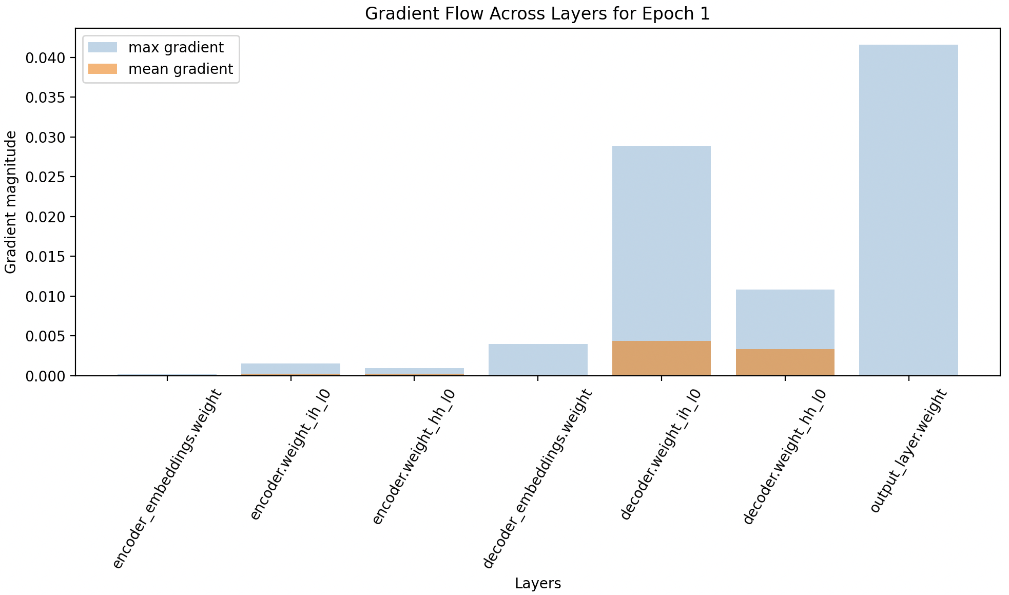
This figure is a classic example telling us that decoder weights, output layers weights are learning or even getting signals from loss but the encoder weights are negligible to see and its not learning anything. Decoders are doing the heavy lifting, when in reality encoder should be the one doing that. Using the visualization, we can see whether gradients are flowing across layers, using max and mean gradients.

Gradient Tracking at each time step

In sequence models like RNNs, learning happens not just across layers but also across time steps. This technique tracks how gradients propagate backward through time, helping us understand whether earlier time steps (which contain long-term dependencies) are being learned effectively. Typically, gradients weaken as they move further back in time, leading to vanishing gradients for long sequences. By visualizing gradient norms per time step, we can observe this decay and assess the model’s ability to capture long-range dependencies. This answers: “Is the model learning from earlier parts of the sequence?”

class TranslationV0(nn.Module):
    """
    Encoder - Decoder Architecture using RNN and context vector - Version 0
    """
    def __init__(self, encoder_emb_dim, decoder_emb_dim):
        super().__init__()
        hidden_size = 10
        #Encoder
        self.encoder_embeddings = nn.Embedding(len(vocab_en), encoder_emb_dim)
        self.encoder = nn.RNN(input_size=encoder_emb_dim, hidden_size=hidden_size, num_layers=1, batch_first=True)
        #Decoder
        self.decoder_embeddings = nn.Embedding(len(vocab_de), decoder_emb_dim)
        self.decoder = nn.RNN(input_size=decoder_emb_dim, hidden_size=hidden_size, num_layers=1, batch_first=True)
        self.output_layer = nn.Linear(in_features=hidden_size, out_features=len(vocab_de))

        #Tracking gradients of RNN and store its hidden vector at each time step
        self.decoder_outputs = None

    def forward(self, encoder_inp, decoder_inp, enc_ip_lengths, dec_ip_lengths):
        #enc_inp : (B, S), dec_inp :  (B, S)
        encoder_emb = self.encoder_embeddings(encoder_inp) #B, S, emb_dim
        out, hidden = self.encoder(encoder_emb) #(B, S, hidden_size), (L, B, hidden_size)        

        decoder_emb = self.decoder_embeddings(decoder_inp)#B, S, emb_dim
        out, hidden = self.decoder(decoder_emb, hidden)  #(B, S, hidden_size), (L, B, hidden_size
        # To visualise whether gradients flow back to each time step in encoder - retain gradients and store the outputs
        self.decoder_outputs = out
        self.decoder_outputs.retain_grad()
        
        logits = self.output_layer(self.decoder_outputs) #(B, S, vocab_size)
        return logits

loss.backward()

#-------------------------- Plot gradient across time steps  --------------------------

# Check for gradients in each time step of the decoder model
grad = model.decoder_outputs.grad
grad_norm_per_timestep = grad.norm(dim=2).mean(dim=0).detach().cpu()
flow = "decoder"

plt.figure()
plt.plot(grad_norm_per_timestep)
plt.xlabel(f"{flow} Time Step")
plt.ylabel("Gradient Norm")
plt.title(f"Gradient Decay Across {flow} Timesteps")
plt.show()

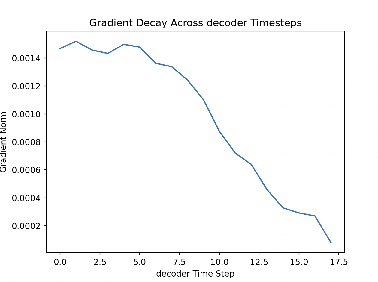
In Decoder : This shows gradients at low steps are very higher than that of far time step. Early decoder states influence many future outputs Their gradients accumulate and give larger gradient norms. While later decoder states influence fewer outputs and smaller gradients

How to Stimulate and Solve Vanishing and Exploding gradients ?

If you guys are curious to learn how to stimulate these problems and solve them below are the few steps you can give a try:

Take your existing LSTM or vanilla RNN and:

1. Use long sequences - 200, 300, 500
2. Increase hidden size (256 or 512)
3. Increase learning rate (e.g., 0.1, 0.5 or 1.0)
4. Initialize weights with large variance. Initialize weights with Normal distribution (mean=0, std=5.0). Large initial weights → large activations → large gradients.

In order to solve these problems :

1. For exploding gradients, clip the gradient norms
2. Better Weight Initialization using Xavier/He initialization for both vanishing and exploding gradients
3. Layer Normalizations for RNN
4. Use Better Architectures like LSTM / GRU
5. Orthongonal Initialization

torch.nn.utils.clip_grad_norm_(model.parameters(), max_norm=1)

torch.nn.init.orthogonal_(rnn.weight_hh_l0)

Hope this blog shared you some useful knowledge!! Happy coding.