Sentiment Classification — Prashanthi's Blog

Welcome to my blog. This is my first Recurrent Neural network on Text data. This project is purely for learning purposes and learning from mistakes.

Brief overview about the Project : It’s a sentiment classification system that is deployed end to end. Dataset is available in Sentiment Classification Dataset Kaggle. Basically we have input sentences and we aim to predict the sentiment of the text which can be either negative, neutral or positive.

Sample of Dataset :

tweet	Sentiment
The event starts at 5 PM.	neutral
I hate how this turned out.	negative
Fantastic experience!	positive

Let’s get into the code:

The idea is to split the datasets into train, validation and test. For sequences / textual data, we have to do some processing. A neural network or any kind of AI system will accept inputs as numbers and we can’t even send characters as input, let alone sentences. First step is to build a vocabulary, like the literal meaning we are building a lookup table to map the words present in our dataset to numbers which will be processed by the model.

Building a vocabulary, its a best practise to use special tokens like “PAD” [ A padding token to fill the samples of differnt lengths in a a batch of data] and “UNK” to handle unseen words of training data.

df = pd.read_csv('tweet_sentiment.csv')
train_df, val_df, test_df = df.iloc[:600], df.iloc[600: 900], df.iloc[900:]

def build_vocabulary(texts: List[str], min_freq = 1):
    tokenized_texts : List[List[str]] = [tokenizer(text) for text in texts]

    counter = Counter()
    for tokenized_text in tokenized_texts:
        counter.update(tokenized_text)

    vocab = {"<PAD>" : 0, "<UNK>" : 1}

    #The idea behind min frequency is in large datasets with noise, typos. Using all the tokens will explode the size of vocabulary
    #Control the items in vocabulary by adding only the tokens with some notable frequency

    for token, freq in counter.items():
        if freq >= min_freq:
            vocab[token] = len(vocab)

    return vocab


token_to_id = build_vocabulary(train_df['tweet'].to_list()) #Use only the training set to build the vocabulary as using other data is leakage
vocab_size = len(token_to_id)
print(f"Size of vocabulary is {vocab_size}")

So far we have only collected the unique words present in our data, we still have to map the words to its numbers. We have to build individual datasets for all three dataframes. Using dataloaders, we have to batch samples of 32 as inputs to the model. While batching we have to do a series of steps:

For each sentences/ instance / sample of a dataset - we must tokenize it. It’s a fancy word, meaning we are going to break down data into its atomic units that coveys meaning to the model. As humans, when we read a sentence, we read word by word to understand the meaning so similarly the neural network at each time step will see a single word.
Once tokenized (Sentence is broken down into list of words) - we must encode it using our vocabulary[ Numericalize - assign numeric value to a token ].
Our samples will be of varying sizes - we must pad the samples of a batch with pad tokens added to match the maximum length of sample in a batch. This is dynamic padding. Back in the day, people used fixed length padding which is inefficient if we look now. For example setting max length as 512 due to sample in X batch, but the maximum length of samples in Y batch is 10, we are wasting of memory and compute due to this inefficiency.

Also map your labels to integers and give tensors. This process is preparing our data ready for model.

class SentimentDataset(Dataset):
    def __init__(self, df):
        super().__init__()
        self.df = df

    def __getitem__(self, idx):
        row = self.df.iloc[idx]
        text = row['tweet']
        label = row['sentiment']
        return text, label

    def __len__(self):
        return self.df.shape[0]

def tokenizer(text:str):
    tokens : List[str] = text.lower().split()
    return tokens

def numericalize(tokenized_text: List[str], vocab:Dict[str,int]):
    encoded = [vocab.get(token, vocab.get("<UNK>")) for token in tokenized_text]
    return encoded


def collate_fn(batch : List[tuple[str, str]], vocab):
    texts, labels = zip(*batch)
    tokenized_texts = [tokenizer(text) for text in texts]
    encoded = [numericalize(tokenized_text, vocab) for tokenized_text in tokenized_texts]
    max_len = max(len(seq) for seq in encoded)
    padded = [
        seq + [vocab["<PAD>"]] * (max_len - len(seq))
        for seq in encoded
    ]
    labels_map = {'negative' : 0, 'neutral' : 1, 'positive' : 2}
    labels = [labels_map.get(label) for label in labels]

    return torch.tensor(padded), torch.tensor(list(labels), dtype=torch.long)

torch.manual_seed(1243)

train_dataset = SentimentDataset(train_df)
val_dataset = SentimentDataset(val_df)
test_dataset = SentimentDataset(test_df)

train_loader = DataLoader(train_dataset, batch_size=32, collate_fn=lambda batch : collate_fn(batch, token_to_id))
val_loader = DataLoader(val_dataset, batch_size=32, collate_fn=lambda batch : collate_fn(batch, token_to_id))
test_loader = DataLoader(test_dataset, batch_size=32, collate_fn=lambda batch : collate_fn(batch, token_to_id))

Next step is obvious, Lets build our neural network, define a loss and optimizer. In order to understand this structure, we must have deep understanding about embeddings and LSTM layer.

nn.Embedding is a learnable layer that provides an embedding vector for each token Id in a sample. This layer under the hood develops a large matrix of size (vocab_size, embedding_dim) which store a dense vector for each token in the vocabulary. This dense vectors are learned during training and they represent the semantic meaning of token. If two tokens are similar (orange, apple) then their corresponding embedding vectors are closer in the vector space. What would break if we fail to use this layer? we can feed raw numbers for each token (say - 100 for orange and 23 for apple) but there is no information to tell that both these terms belong to fruits category. In order to capture the semantic meaning, we build a high dim dense vector called embedding vector for each token using a learnable fancy lookup table ( of size vocab_size * embed_dim )

LSTM cell is a special cell preserving two states - cell state (long term memory) and hidden state (short term memory).This cell itself deserves a entire blog post so I am skipping it here.

The loss function that is used for this task is Cross entropy loss which accepts raw logits of the model and targets as class indices. It is expected for the logits to be of float datatype and class indices of long datatype(int64). This datatype mismatch got me stuck for hours, so watch out. Like every models, do not get the prediction labels and feed to the loss function. I have used SGD as optimizer and it performed better.

class LSTMModel(nn.Module):
    def __init__(self, size, embedding_dim, output_size, hidden_size):
        super().__init__()
        self.embedding = nn.Embedding(size, embedding_dim)
        self.lstm = nn.LSTM(embedding_dim, hidden_size, batch_first=True)
        self.output_layer = nn.Linear(hidden_size, output_size)

    def forward(self, x):
        x, (hidden, cell) = self.lstm(self.embedding(x)) # x -> (B, S, H) , hidden -> (1, B, H)
        out = self.output_layer(hidden.squeeze(0)) 
        return out


model = LSTMModel(vocab_size, 100, 3, 64)
loss_fn = nn.CrossEntropyLoss()
optimizer = torch.optim.SGD(params=model.parameters(), lr=0.01)

One of the best practise is to always predict on a single sample before training, so we can see how a model works on randomized weights. Then we train it for our dataset, penalize it for the mistakes it does, optimize the parameters it holds. After training, we can call same the predict on the sample sample, but this time the model would have learned and makes correct predictions.

#Before Training
first_batch_X, first_batch_y = next(iter(test_loader))
print(first_batch_X.shape, first_batch_y.shape)

encoded_text, sentiment = first_batch_X[3:4], first_batch_y[3:4]
id_to_token = {token_id : token for token, token_id in token_to_id.items()}
reverse_labels_map = {0 : 'negative', 1 :  'neutral', 2 :  'positive'}

decoded_text = [id_to_token.get(token_id.item()) for token_id in encoded_text[0]]
print(decoded_text)
print(f"First sample :: {" ".join(decoded_text)}")
out = model(encoded_text).argmax(dim=1).item()
print(f"Model prediction : {reverse_labels_map.get(out)}, Actual sentiment : {reverse_labels_map.get(sentiment[0].item())}")

Some code above is written for understanding the encoded text, raw prediction and actual sentiment. But the important part of above code is called model(seq) which is the forward pass.

Next comes the heavy-lifting, we train our model, note down the training and validation loss. Additionally for each batch we compute the accuracy to visualize those as well. If you are aware of the mechanics of one training step, then the below code is cake walk, no matter how length it looks.

One Training step : [Training Mode]

Forward pass : model(X_Batch)
Compute loss : loss = loss_fn(logits, y_batch)
Reset the optimizer gradients : optimizer.zero_grad()
Backward pass : loss.backward()
Update the parameters with the gradients computed : optimizer.step()

For Evaluation mode

Forward pass : model(X_Batch)
Compute loss : loss = loss_fn(logits, y_batch)

Important thing is to set the model’s state using train() and eval(). Also using torch.inference_mode() warns the autograd engine to not compute the computation graph thus optimizing a lot of stuff for us so the inference is faster.

Additional stuff I did:

-> I have computed loss and accuracy for each batch, for each step in order to plot the loss and accuracy for each epoch. Purely visualisation purposes. -> The assert statements I have added is a good practise for any pipelines. We have this broadcasting issues when we perform operations on predicted and true labels if sizes don’t match. It’s often required to check shapes to avoid miscalculations. -> Use detach() on loss because we don’t want to add new nodes on computation graph.

def accuracy(y_true, y_pred):
    return (y_true == y_pred).float().mean()

train_loss, train_acc, val_loss, val_acc = [], [], [], []
num_epochs = 20
for epoch in range(num_epochs):
    train_loss_per_step, train_acc_per_step, val_loss_per_step, val_acc_per_step = [], [], [], []
    model.train()
    for X_batch, y_batch in train_loader:
        logits = model(X_batch)
        loss = loss_fn(logits, y_batch)

        y_pred = logits.argmax(dim=1)
        assert y_pred.shape == y_batch.shape

        train_loss_per_step.append(loss.detach().item())
        train_acc_per_step.append(accuracy(y_batch, y_pred).item())

        optimizer.zero_grad()
        loss.backward()
        optimizer.step()

    model.eval()
    with torch.inference_mode():
        for X_batch, y_batch in val_loader:
            logits = model(X_batch)
            loss = loss_fn(logits, y_batch)

            y_pred = logits.argmax(dim=1)
            assert y_pred.shape == y_batch.shape

            val_loss_per_step.append(loss.detach().item())
            val_acc_per_step.append(accuracy(y_batch, y_pred).item())

    train_loss.append(torch.tensor(train_loss_per_step).mean())
    train_acc.append(torch.tensor(train_acc_per_step).mean())
    val_loss.append(torch.tensor(val_loss_per_step).mean())
    val_acc.append(torch.tensor(val_acc_per_step).mean())

    if epoch % 1 == 0:
        print(f" For epoch : {epoch}/{num_epochs}, Train Loss : {train_loss[-1]:.2f}"
                f" Train Acc : {train_acc[-1]:.2f}, Val Loss : {val_loss[-1]:.2f}, Val acc : {val_acc[-1]:.2f}")

Visualization Loss vs Accuracy curves

epochs_range = range(1, num_epochs + 1)
fig, axes = plt.subplots(1, 2, figsize=(10, 7))

axes[0].plot(epochs_range, train_loss, label = "Train Loss")
axes[0].plot(epochs_range, val_loss, label = "Validation Loss")
axes[0].set_xlabel("Epochs")
axes[0].set_ylabel("Loss")
axes[0].set_title("Epochs vs Loss")
axes[0].legend()

axes[1].plot(epochs_range, train_acc, label = "Train Accuracy")
axes[1].plot(epochs_range, val_acc, label = "Validation Accuracy")
axes[1].set_xlabel("Epochs")
axes[1].set_ylabel("Accuracy")
axes[1].set_title("Epochs vs Accuracy")
axes[1].legend()

plt.tight_layout()
plt.savefig("acc_loss_plots.png")
plt.show()

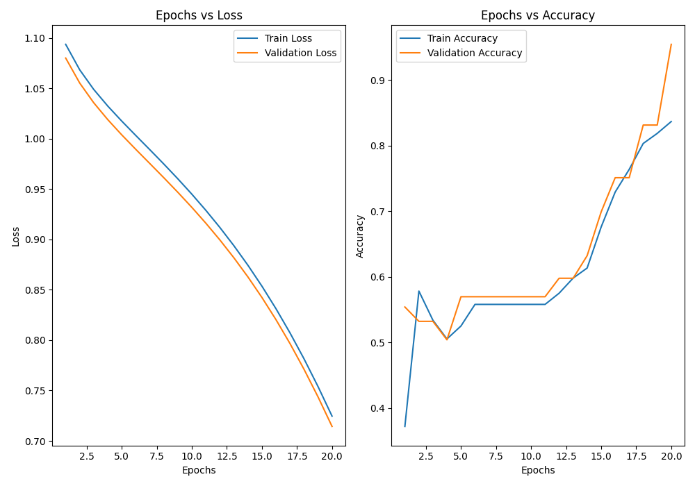
Our model clearly learned over epochs, you can see this with the falling curves in Loss plot and rising curves in accuracy plots. Let’s move to move evaluation, check how well our model performs on the test set and Also verify whether our single sample is predicting correctly now that the model is trained.

#After Training
first_batch_X, first_batch_y = next(iter(test_loader))
encoded_text, sentiment = first_batch_X[3:4], first_batch_y[3:4]
id_to_token = {token_id : token for token, token_id in token_to_id.items()}
reverse_labels_map = {0 : 'negative', 1 :  'neutral', 2 :  'positive'}

decoded_text = [id_to_token.get(token_id.item()) for token_id in encoded_text[0]]
print(f"First sample :: {" ".join(decoded_text)}")
out = model(encoded_text).argmax(dim=1).item()
print(f"Model prediction : {reverse_labels_map.get(out)}, Actual sentiment : {reverse_labels_map.get(sentiment[0].item())}")

test_loss , test_acc= [], []
model.eval()
with torch.inference_mode():
    for X_batch, y_batch in test_loader:
        y_pred = model(X_batch)
        loss = loss_fn(y_pred, y_batch)

        y_pred = y_pred.argmax(dim=1)
        assert y_pred.shape == y_batch.shape

        test_loss.append(loss.detach().item())
        test_acc.append(accuracy(y_batch, y_pred).item())

print(f"Test Loss : {torch.tensor(test_loss).mean():.2f}, Test Accuracy : {torch.tensor(test_acc).mean():.2f}")

torch.save(model.state_dict(), "model_weights.pth")
with open('vocab.json', 'w') as f:
    json.dump(token_to_id, f)

Save your pytorch model weights and the vocabulary json, because the next step we are going is to see is inference. Inference is the single most important thing out of the entire pipeline. If you can’t predict on unseen data, there is no purpose in training a NN. Create a file namely inference.py and app.py for the streamlit app.

In the inference function, basically we will take a text entired by user in the UI, we will preprocess it same way we did while building a batch in collate fn, we will tokenize, encode and for padding we keep the natural length. Somehow Adding a padding of max_len for a batch of one sample is the length of that sample. Create an instance of your LSTM model and load the pretrained weights. Set to inference mode and start predicting, its that simple.

Setting up FastAPI, an endpoint to receive requests made by the frontend and return results. Creating a Pydantic model for better structurized code and then expose your endpoint.

def preprocess(text: str, vocab):
    tokenized = text.lower().split()
    encoded = [vocab.get(token, vocab.get("<UNK>")) for token in tokenized]
    padded_seq = encoded
    return torch.tensor(padded_seq).unsqueeze(0) #(1, max_len)


def get_inference(text:str):
    with open('vocab.json', 'r') as f:
        vocab = json.load(f)
    sequence = preprocess(text, vocab)

    model = LSTMModel(len(vocab), 100, 3, 64)
    model.load_state_dict(torch.load('model_weights.pt'))

    results = None
    model.eval()
    with torch.inference_mode():
        raw_logits = model(sequence)
        y_pred = raw_logits.argmax(dim=1).item()
        reverse_labels_map = {0 : 'negative', 1 :  'neutral', 2 :  'positive'}
        results = {'prediction' : reverse_labels_map.get(y_pred)}

    return results

# pip install fastapi uvicorn
# uvicorn inference:myapp --reload
myapp = FastAPI()

class TextInput(BaseModel):
    text : str

@myapp.post("/predict")
def predict(data : TextInput):
    prediction = get_inference(data.text)
    return prediction

Let’s move to the streamlit app, run your fast api using the below command

uvicorn inference:myapp --reload

You can see the endpoint where your API is exposed, create your streamlit app and run it

streamlit run app.py

import streamlit as st
import requests

st.title("Sentiment classifier")
user_input = st.text_area("Enter the text: ")

if st.button("Predict"):
    with st.spinner("Predicting..."):
        response = requests.post("http://127.0.0.1:8000/predict", json={"text" : user_input})
        if response.status_code == 200:
            response = response.json()
            print(response)
            prediction = response["prediction"]
            st.success(f"Prediction results {prediction}")
        else:
            st.error("Error in loading results")

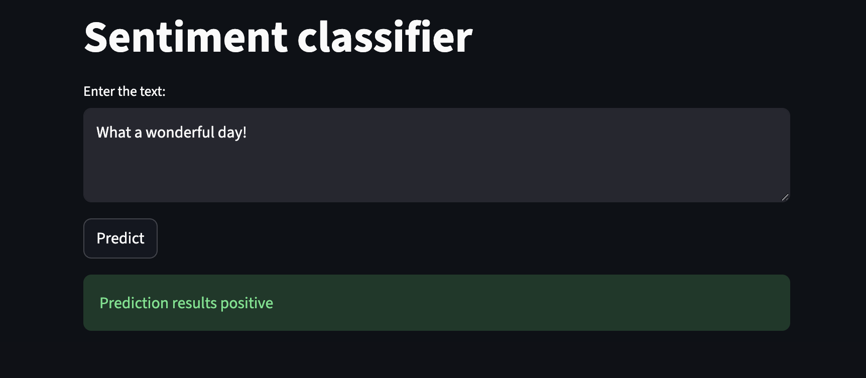
Positive sentiment case:

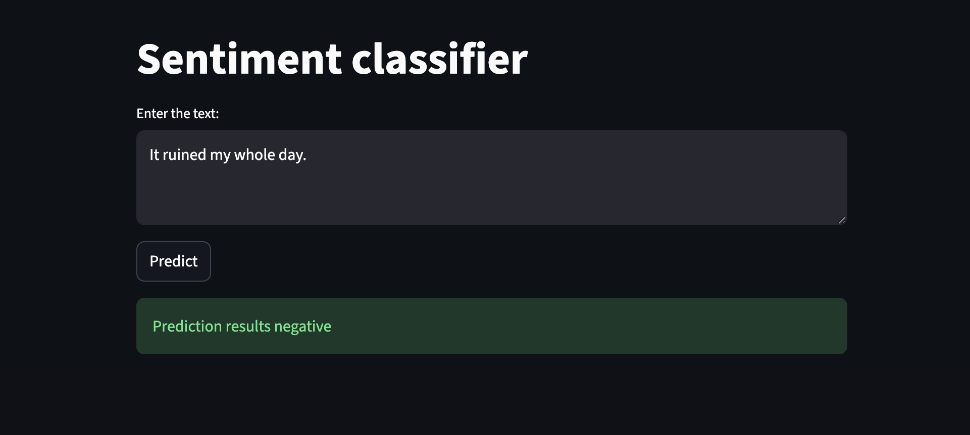
Negative sentiment case:

Finally I would like to end with the limitations of my model. If we give words outside of my vocabulary( there are only 66 words in my vocab )then the prediction is inaccuracte.