Hello everyone, this is a sequel to my previous blogs. I started understanding architectural advancements in the deep learning field from RNNs to Seq2Seq and then to attention mechanisms, finally we are landing on Transformers. Throughout this journey, I was focussed on one task, a simple task namely reverse a sequence of numbers and produce a sequence of numbers. The reason why I chose this is, this strips us down the data layer and helps us focus on the architecture layer. We would never reach the stage where we say, data is not enough or compute is not enough. We can easily scale our data based on the compute is available and this task helps us see the architectures transparently. Before getting into transformers, we should know what limitations we faced before. Previously using recurrence we solved sequence to sequence problems, but the difficulty we faced is they are sequential in nature, unstable training due to vanishing and exploding gradients, long term dependencies are not captured. To solve long term dependencies, people introduced attention mechanisms, To truly take advantage of it, people replaced recurrence concept with pure attention algorithms which is transformers. Prerequisites of this blog is to have basic knowledge in Encoder - Decoder architecture.

Check out the most important paper here, we will borrow nice images from it and I will explain it’s meaning in simple terms. Attention is all you need. This entire blog is in reference with the paper. We are breaking down the paper into simple components and also explain Transformers along the way.

Our flow is simple, first we will use the prebuilt blocks present in pytorch, secondly we will understand what these blocks mean separately, finally we will build our transformers architecture from scratch.

Building Transformers using Pre-built blocks in Pytorch

In the paper, page 3, figure 1, We have transformers architecture which may look complicated at once but in simple terms it is made up of 5 blocks as follows,

1. Embedding Layer
2. Positional Encoding Layer
3. Encoder block repeated N times, present in left side of architecture
4. Decoder block repeated N times, present in right side of architecture
5. Output layer

I have used all these blocks in 6 to 7 lines to build my transformers architecture.

class ReverseTaskV9(nn.Module):
    """
    Transformer architecture from "Attention is all you need" paper using pre-built transformer blocks
    """
    def __init__(self, d_model):
        super().__init__()
        self.input_embeddings = nn.Embedding(VOCAB_SIZE, d_model)
        self.pos_input_embeddings = nn.Embedding(MAX_LEN, d_model)
        self.encoder_layer = nn.TransformerEncoderLayer(d_model=d_model, nhead=4, dim_feedforward=128, batch_first=True)
        self.encoder = nn.TransformerEncoder(self.encoder_layer, num_layers=2)

        self.output_embeddings = nn.Embedding(VOCAB_SIZE, d_model)
        self.pos_output_embeddings = nn.Embedding(MAX_LEN + 1, d_model)
        self.decoder_layer = nn.TransformerDecoderLayer(d_model=d_model, nhead=4, dim_feedforward=128, batch_first=True)
        self.decoder = nn.TransformerDecoder(self.decoder_layer, num_layers=2)

        self.output_layer = nn.Linear(d_model, VOCAB_SIZE)

    def forward(self, enc_inps, dec_inps):
        B, S = enc_inps.shape  # S - source seq len
        enc_position_ids = torch.arange(0, S).unsqueeze(0).repeat(B, 1)
        enc_token_embeddings = self.input_embeddings(enc_inps) # (B, S) -> (B, S, D )
        enc_pos_embeddings = self.pos_input_embeddings(enc_position_ids) # (B, S) -> ( B, S, D)
        enc_embeddings = enc_token_embeddings + enc_pos_embeddings # ( B, S, D ) + ( B, S, D ) = ( B, S, D)
        enc_outputs = self.encoder(enc_embeddings) # (B, S, D)

        B, T = dec_inps.shape #T - Target seq len
        dec_position_ids = torch.arange(0, T).unsqueeze(0).repeat(B, 1)
        dec_token_embeddings = self.output_embeddings(dec_inps) # (B, T) -> (B, T, D)
        dec_pos_embeddings = self.pos_output_embeddings(dec_position_ids) # (B, T) -> (B, T, D)
        dec_embeddings = dec_token_embeddings + dec_pos_embeddings  # ( B, T, D ) + ( B, T, D ) = ( B, T, D)
        tgt_mask = nn.Transformer.generate_square_subsequent_mask(T)
        dec_outputs = self.decoder(dec_embeddings, enc_outputs, tgt_mask = tgt_mask) # ( B, T, D), (B, S, D) -> ( B, T, D)

        logits = self.output_layer(dec_outputs) # ( B, T, D) -> (B, T, V)
        return logits

Let’s untangle each block of line,

1. Embedding layer - Both the encoder inputs and decoder inputs must go through a embedding layer ( Vocabulary lookup table ) to capture the semantic meaning of a token. In code, it takes a token ID and results a n-dimensional vector representing the semantic meaning of the token. For example, it takes cat and maps a n-dim vector.
2. Positional Encoding - The major upgrade in transformers is that, it doesn’t process tokens sequentially. In our system, it doesn’t know the order of words. For the encoder/decoder it looks like a bag of words. One way to solve this problem is to inject the positional meaning into our architecture. We are using another embedding layer which now maps raw position ids as 1, 2, 3 to a vector. Together both the vectors from both the embedding layer is added and sent to our Encoder/Decoder.
3. Encoder : If you look in our paper, figure 1, Encoder is combination of multi-head self attention and feed forward network. We also have residual connections and normalization layers placed after both of these blocks.
   • The purpose of residual connections, is to remember the original signal before the transformation and learn the necessary changes to apply on original signal and produce output. Without this, we would give original signal and ask the model to build output from scratch. Think of it like this, inputs are the hint to generate outputs, tweaking inputs will give us outputs and that is what we are trying to achieve in skip/residual connections
   • The purpose of layer norm, is to control the signals from getting too large, too small or unstable across layers. We will look closely on multi-head attention and feed forward in later parts.
4. Decoder : Decoder is the combination of masked multi-head self attention, multi head cross attention and feed forward network. Decoder is made up of 3 small blocks with skip connections and layer norm interleaved.
5. Output Layer : This layer takes all the predictions of the decoder and map it to the vocabulary to get the maximum likelihood token and return that token as next word prediction.

In pytorch, we create the encoder/decoder layer and then pass it the Transformer encoder with the number of layers mentioned to create the N * Encoder layer block. Encoder = N * Encoder Layer

Individual Blocks of Transformers

Positional Encoding

In our pre-built code we have used embedding layer to get positional information, but in the paper they have used a formula (sine and cosine based) and directly generating the vector for each position instead of using an embedding layer / extra parameters. Check out section 3.5 for the formula and below is it corresponding torch implementation.

def positional_encoding(pos, d_model):
    assert d_model % 2 == 0
    pe = torch.zeros(pos, d_model) #(pos, d_model)
    
    positions = torch.arange(0, pos).unsqueeze(1) #(pos, 1)
    index = torch.arange(0, d_model, 2) #(d_model/2, )
    
    freq = torch.exp(index * (- math.log(10000.0)/ d_model))  #(d_model/2, )
    pe[:, 0::2] = torch.sin(positions * freq) #(pos, 1) * (d_model/2,) → (pos, d_model/2)
    pe[:, 1::2] = torch.cos(positions * freq) #(pos, 1) * (d_model/2,) → (pos, d_model/2)

Why sine & cosine?

Because they have a special property. From two positions’ encodings, the model can easily figure out relative distance

Instead of learning positions (like embeddings), the paper creates them using: Waves (sine & cosine) of different frequencies. Each position is encoded as a combination of waves: Some dimensions change very fast, Some change very slowly, So each position gets a unique “wave signature”.

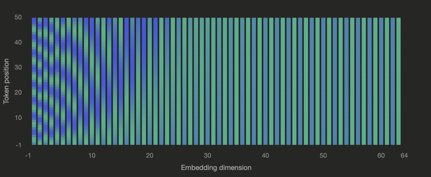
In the above image, dimensions like 0 to 10 change so fast showing relative distances in closer position ids. But for dimensions above 30 the values are almost same but behind the scenes its slowly changing. In the y-axis, we have only 50 position ids, if we increase to 200, 300 then the values change across later dimension like 60, capturing long range positional differences.

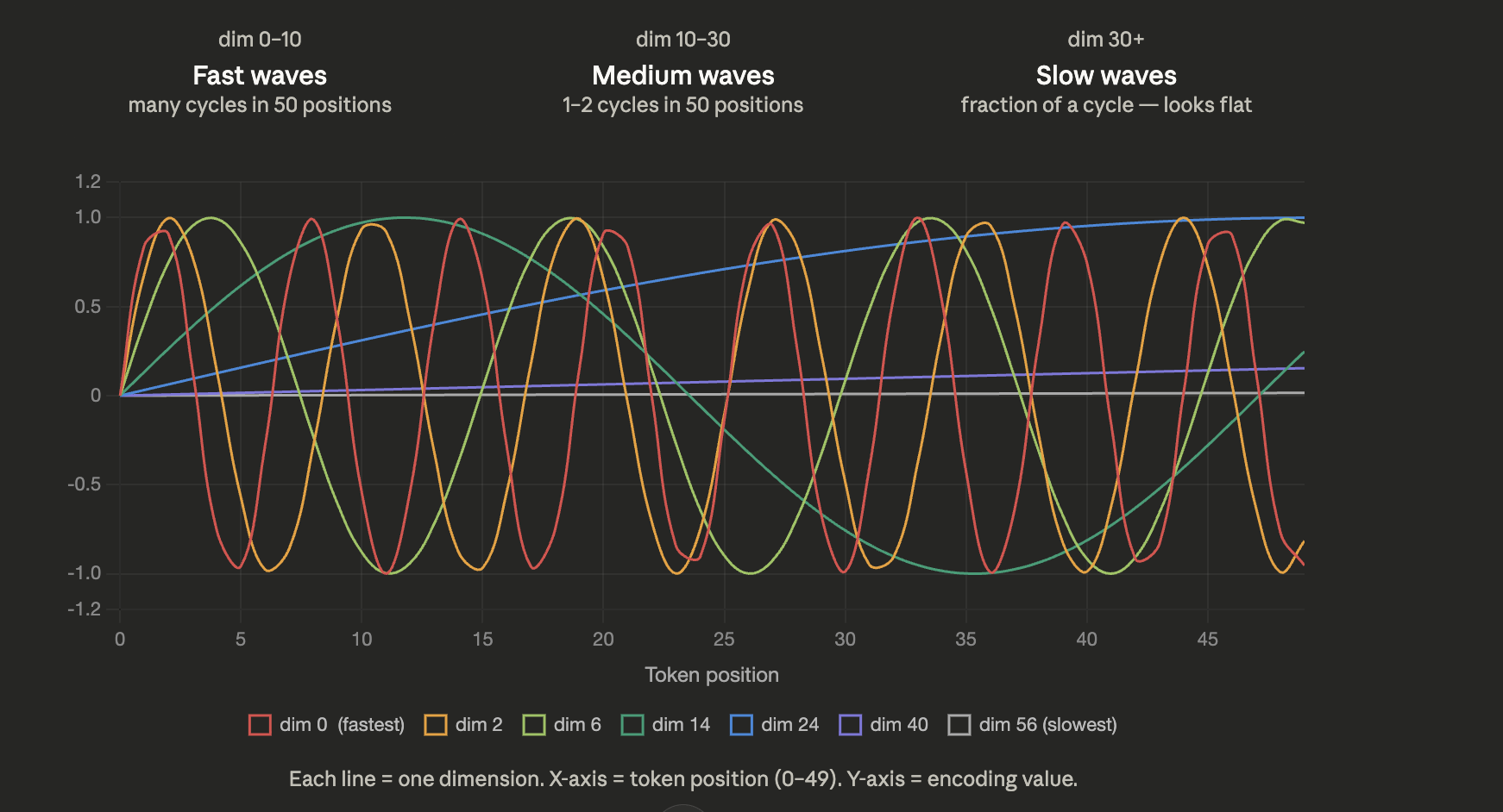
From the above image, take dim=0, its wave is fast and values repeat the same for every 5 position ids, whereas dim=14 values repeat every 40 position ids. Each dimension is a wave of its own frequency. We have fast wave is early dimensions and slow waves in latter dimensions. As the count of words in your sentence increases, your vector dimensions must increase as well to learn the patterns in positions of farther words. Enough of intuition, let’s get into the code snippet.

1. Inputs (pos, d_model) where pos is number of words (how many positions) and d_model is the size of each positional vector
2. Output (pe) of shape (pos, d_model) where each row is a positional encoding of a word
3. Positions tells where we are (0,1,2,3…) and index tells which dimension we are filling. Each dimension represents a wave with a different frequency.
4. Frequency term creates a fast wave for slow index and slow wave for fast index. So each dimension behaves differently.
5. For each position, we plug it into waves of different frequencies by calculating its sine and cosine versions. Remember sin and cos are same waves but shifted. This gives us 2 views of same positon.

Each position is encoded as a combination of sine and cosine waves at different frequencies, so that every position gets a unique pattern and the model can easily learn relative distances between positions.

Scaled Dot product attention.

If you look at the transformer architecture in section 3.1, we have crossed the positional encoding stage and the first block we have is Multi-head Attention.

Take a sentence : “The cat sat on the mat”

Our Tokens are : [“The”, “cat”, “sat”, “on”, “the”, “mat”]. For understanding purposes we are considering words, but the model sees only vectors representing words. Now our vectors hold both semantic meaning and positional meaning.

As you can look in the figure, we take the input and repeat it as 3 parameters and send to the multi-head attention block. These parameters are Queries, Keys, Values and for this case as per diagram all the three inputs are same list of tokens.

Query (Q): what am I looking for? Key (K): what do I contain? Value (V): what information should I pass? Refer the section 3.2.1 as we explore this block.

As you can see Multi head attention is a combination of scaled dot-product attention so let’s check it out. Simultaneously look at the left diagram of figure 2 and the following code snippet as you follow the steps after it,

def scaled_dot_product_attention(Q, K, V, mask=None):
    similarity_scores = Q @ K # [[0.1, 0.2, 0.3 ...] -> "The", [0.2, 0.3, 0.5, .. ] -> "cat" ...]
    d_k = K.shape[2]
    scores = similarity_scores / math.sqrt(d_k) 
    if mask is not None :
        scores = scores.masked_fill(mask == 0, -1e9) 
    attention_weights = torch.softmax(scores, dim=-1) 
    output = attention_weights @ V 
    return output, attention_weights

1. Matrix multiplication of Queries and Keys. Matrix multiplication is dot product of tokens in a sentence with itself across a batch of sentences. We compute dot product of each token in our list with itself telling how similar queries and keys are with each other. For example, similarity scores is now a list of list of numbers, “The” token is changed as doct products of “The” with every other token in the list
2. To avoid similarity scores/ dot products from growing two large we scale down all the values. This scaling is purely for stablizing similarity scores.
3. Mask is optional and it is provided to our function. Mask turns some similarity scores into high negative values thus later when we exponentiate in softmax, it gets zero. We are smartly turning off the attention for some words based on mask.
4. We turns this scores to probabilities by calling softmax, Now for the “The” list of scores, it now contains probabilities saying how similar “The” word is with other word in the sentence.
5. Remember values are our same list of tokens, we take this values and multiply our probs. So for “The” the list of probabilities is multiplied with the words, such that “The” representation is now a combination of all the words in the sentence weighted by the similarity probs we found. “The” is no more a single word but a richer representation of the entire sentence/entire context.

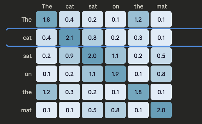
Check out the similarity scores matrix that we generated in first step. It gives scores on how much two tokens are related.

Multi Head Attention

Instead of performing attention once, we perform it multiple times in parallel, using different heads.

1. We start with input vectors (which already contain semantic + positional information).
2. We apply linear projections to generate Q, K, V. We are allowing them to undergo different perspectives before we compute attention
3. Instead of using these directly, we split them into multiple heads. Example our vector is 512 dim meaning d_model = 512, if n_heads = 8 then each head 64 dim. Instead of computing one attention on 512 dim vector, we allow different heads to work on smaller representation.
4. Note the subtle thing we transpose dimensions in our splitting heads section. Previously each word had its head, but we wanted heads across all tokens, so we transpose. Each head looks at all words and trying to learn different pattern to minimise loss.
5. Scaled dot product attention as explained above.
6. We concatenate all heads and pass through a final linear layer.

class MultiHeadAttention(nn.Module):
    def __init__(self, d_model, n_heads):
        super().__init__()
        self.n_heads = n_heads
        self.d_model = d_model
        self.head_dim = self.d_model // self.n_heads
        self.d_k = self.head_dim

        self.W_Q = nn.Linear(in_features=d_model, out_features=d_model)
        self.W_K = nn.Linear(in_features=d_model, out_features=d_model)
        self.W_V = nn.Linear(in_features=d_model, out_features=d_model)
        self.W_out = nn.Linear(in_features=d_model, out_features=d_model)

    def forward(self, x,  to_mask=False):
        B, T, d_model = x.shape

        #1. Projections( Look at full input → extract features)
        Q = self.W_Q(x) #(B, T, d_model)
        K = self.W_K(x) #(B, T, d_model)
        V = self.W_V(x) #(B, T, d_model)

        #2. Splitting into heads ( Group features into heads )
        Q = Q.view(B, T, self.n_heads, self.head_dim).transpose(1, 2) #(B, T, n_heads, head_dim) -> (B, n_heads, T, head_dim)
        K = K.view(B, T, self.n_heads, self.head_dim).transpose(1, 2) #(B, T, n_heads, head_dim) -> (B, n_heads, T, head_dim)
        V = V.view(B, T, self.n_heads, self.head_dim).transpose(1, 2) #(B, T, n_heads, head_dim) -> (B, n_heads, T, head_dim)

        #3. Scaled Dot product attention (Each head processes its own feature set)
        scores = Q @ K.transpose(-1, -2) # (B, n_head, T, head_dim ) @ (B, n_head, head_dim, T) = (B, n_head, T, T)
        scores = scores / math.sqrt(self.d_k) # (B, n_heads, T, T)
        if to_mask:
            mask = torch.tril(torch.ones(T,T)).unsqueeze(dim=0).unsqueeze(dim=0) #(T, T) ->( 1, T, T) -> (1, 1, T, T)
            scores = scores.masked_fill(mask == 0, -1e9)  # (B, n_heads, T, T)
        attention_weights  = torch.softmax(scores, dim=-1)  # (B, n_heads, T, T)
        out = attention_weights @ V  # (B, n_heads, T, T)  @ (B, n_heads, T, head_dim) = (B,n_heads, T, head_dim)

        #4. Concatenate all heads information
        out = out.transpose(1, 2).contiguous().view(B, T, d_model) #( B, T, n_heads, head_dim ) -> (B, T, d_model)
        return self.W_out(out) #(B, T, d_model)

Each head focuses on a different type of relationship in the sentence. For example:

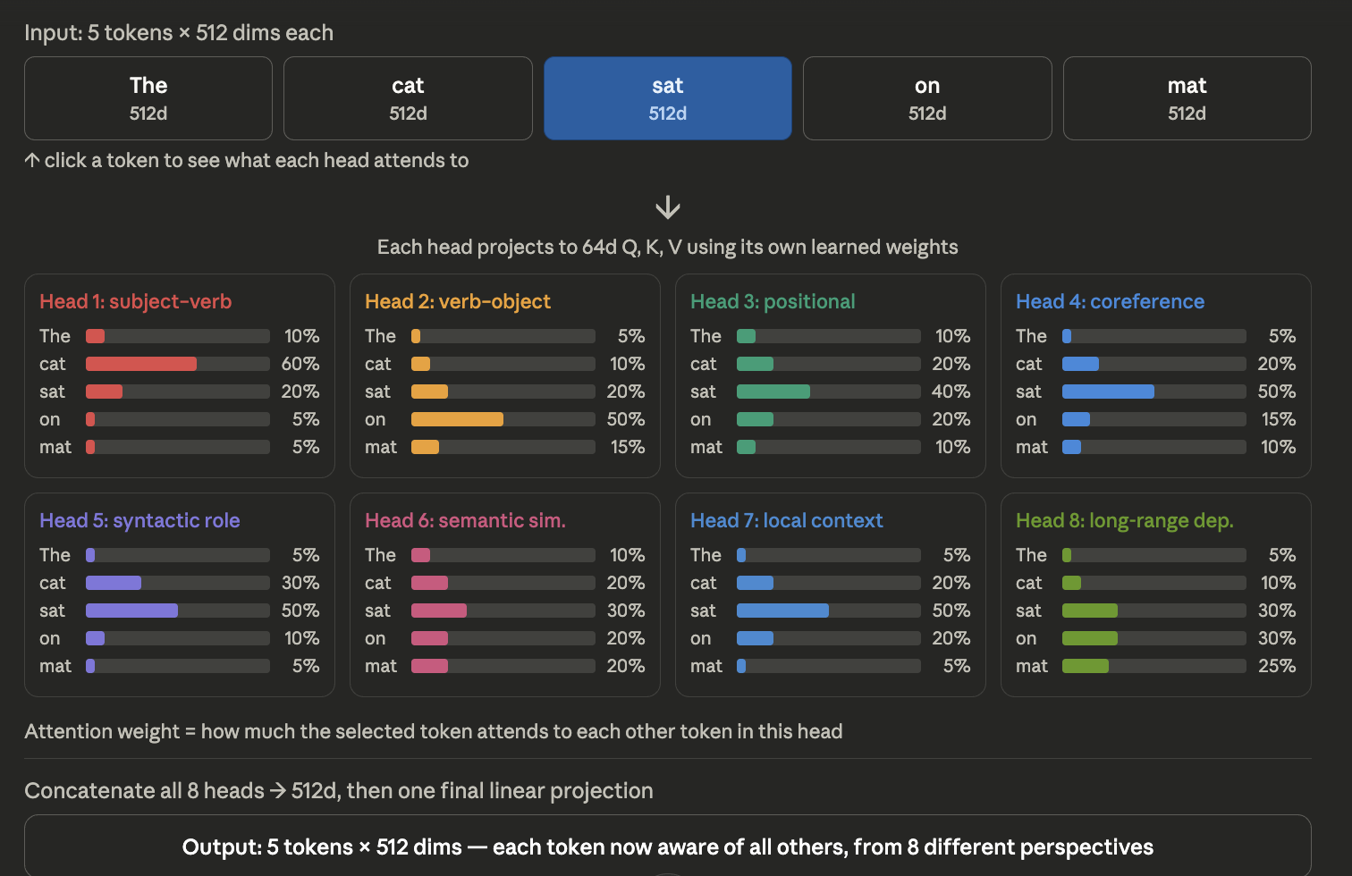
One head may focus on syntax (subject–verb) One head may focus on position One head may focus on semantic similarity. Check out the figure below, for the word “sat”, we our seeing the attention weights of all the tokens in different heads/sub spaces. Heads are trying to look at different perspective and asks different kind of question with its provided subspace for all tokens.

A More Deeper Intuition is given below :

One vector per token. The model splits that vector into 8 dimensional subspaces (64 dims each). Each head looks at all the tokens but only through the lens of its own 64-dim subspace. So head 1 might be asking “what syntactic role does each token play” (using its 64 dims), while head 2 asks “what semantic entities are related” (using a different 64 dims). To be precise: Each head attends over all tokens in the sequence, but computes attention within its own 64-dim subspace. Different heads specialize in different kinds of relationships because they’re looking at different subspace of the same input. Instead of one giant 512-dim attention trying to capture everything at once, you have 8 smaller 64-dim attentions each focusing on a different aspect. Then you concatenate all 8 outputs back into 512 dims.

What’s actually happening is this:

the model is learning a factorization of attention. Instead of “how does token i relate to token j in one giant 512-dim space,” it’s learning “token i relates to token j in 8 different ways simultaneously.” Each head captures one flavor of relationship. Think of a human reading a sentence. You’re not doing one monolithic “understanding.” You’re simultaneously tracking:

Grammar (which words are subjects, verbs, objects), Coreference (“she” refers back to which person?), Semantics (what concepts are related?), Discourse structure (is this a cause, a result, a contrast?). A transformer’s multi-head attention is mimicking that — doing multiple kinds of analysis at once, in parallel, on the same input.

Variants of Attention

Self Attention :

• Queries == Keys [ Queries and keys come from same inputs (Decoder’s inps or Enc’s inps).
• Words attends other words of the same sentence

Cross Attention :

• Queries != Keys [ Queries are decoder inputs and Keys are encoder outputs ].
• Words attends other words of different sentence.

Transformer Architecture from scratch

Check out entire code in github. I can’t display everything here, but I will explain the intuition behind the code here. Most of the code present there is already explained in different blocks of code.

We are trying to understand the intuition behind a different task but same architecture, this time not as a block, we are seeing end to end of figure 1 in paper. Our task here is to reverse a sequence. You give the model [5, 3, 9] and you want it to output [9, 3, 5]. The transformer learns to do this through an encoder (reads the input) and a decoder (writes the output, one token at a time).

Step 1 : Computing Embeddings and Encodings

Your three numbers [5, 3, 9] each get converted into a 64-dimensional vector (a list of 64 floats). Raw numbers gets converted to a vector That’s the token embedding — it’s like a learned representation for each number. Tells the model “what” the token is. Then we add a positional encoding on top( Uses sin/cos waves to encode positions), so the model knows 5 is at position 0, 3 at position 1, 9 at position 2. Tells the model “where” the token is. Without this, a transformer would treat [5, 3, 9] the same as [9, 5, 3].

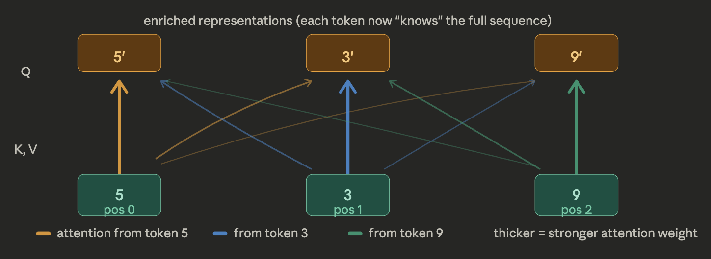
Step 2 : Encoder self attention

Every token asks the question “which other tokens are relevant to me?”. Token 5 produces a Query vector (what am I looking for?) and every token produces a Key vector (what do I offer?). The dot product of Query × Key gives a score. Softmax turns those scores into weights. Then each token blends all other tokens’ Value vectors according to those weights. The result is 5’, 3’, 9’ — these are enriched vectors. Each one now carries information about the whole sequence, not just itself. The thicker the line, the more one token “paid attention” to another. Then each enriched vector passes through a feedforward network.

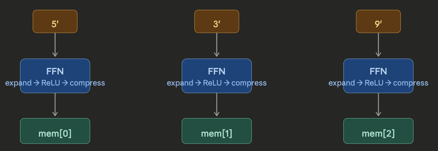
Step 3 : Encoder Feed Forward Network

After attention lets tokens talk to each other, the feedforward network processes each token independently through the same small MLP — expand to 256 dims → ReLU → compress back. It’s the part that does the “thinking” on the enriched representation. The result is your encoder memory: three vectors mem[0], mem[1], mem[2] that represent the full understood context of [5, 3, 9]. This gets passed to the decoder.

The entire encoder block for a single token is depicted in figure below,

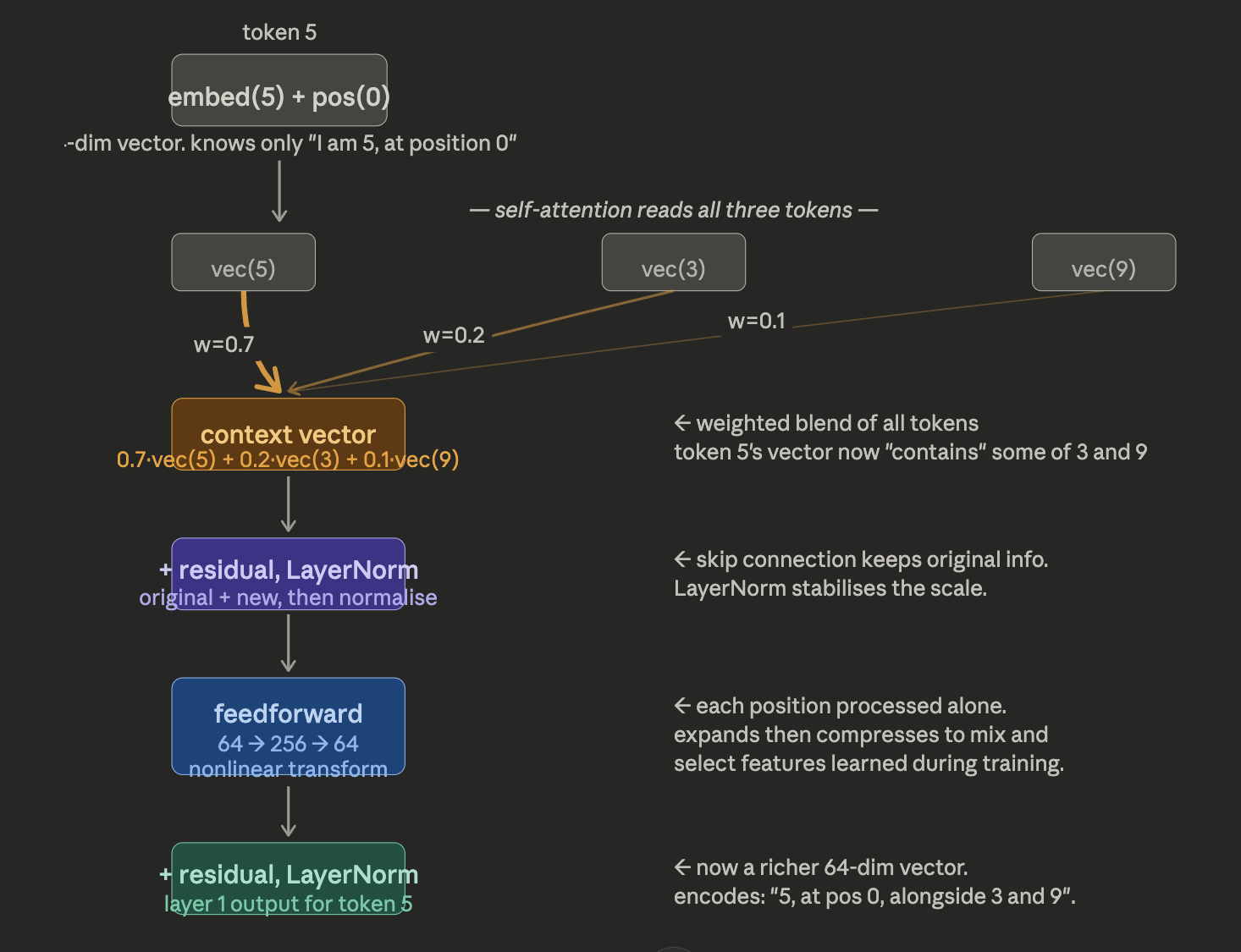
Before any layer: Token 5’s vector says “I am the number 5, and I am at position 0.” That’s it. It knows nothing about 3 or 9 sitting next to it. After self-attention: The attention mechanism computes how much token 5 should “borrow” from each other token. Say the weights come out as 0.7 for itself, 0.2 for token 3, and 0.1 for token 9. The new vector for token 5 is literally a weighted sum — 0.7 × vec(5) + 0.2 × vec(3) + 0.1 × vec(9). The vector for token 5 now has some of token 3 and token 9 mixed into it. It no longer just knows about itself — it has absorbed context from its neighbours. The residual connection: Instead of replacing the old vector, the output of attention is added to the original. So nothing is forgotten. The original “I am 5 at position 0” information is still there, and the new neighbourhood context is layered on top. After the feedforward network: The FFN doesn’t look at other tokens — it processes the vector for token 5 alone. But it expands it to 256 dims, applies a nonlinearity, and compresses back. This lets the model do complex feature transformations — like combining the “I’m a 5” signal with “I have a large neighbour (9)” to produce a higher-level feature that might be useful for the reversal task. With 2 layers (your model has num_layers=2): This whole process repeats. In layer 2, token 5’s vector already contains a blend of the whole sequence from layer 1. So when attention runs again, it’s not just blending raw token identities — it’s blending already-enriched representations. Layer 2 can pick up higher-order patterns, like relative positions across the sequence.

Step 4 : Decoder Masked Multi-head self attention

During training (teacher forcing), decoder sees the correct reversed sequence, shifted right. The decoder gets [SOS, 9, 3] as input (the reversed sequence, shifted right) and predictions need to be [9, 3, 5]. At every position it must predict the next token. Given SOS, model must predict 9, Given 9, model must predict 3, Given 3, model must predict 5,

Why shift right?

at each position, the model predicts the next token using only what came before. SOS is the “start” signal — it has no meaning, just tells the decoder to begin generating

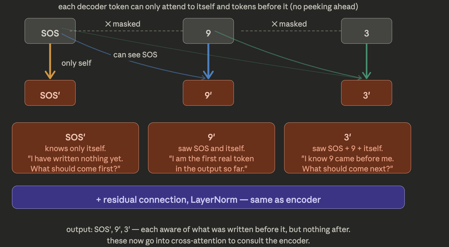
The decoder tokens talk to each other, but only backwards. SOS is completely isolated — it only sees itself. Token 9 can glance back at SOS to understand “I am the first real token written.” Token 3 can see both — it knows the output history so far. This is the “what have I written?” stage. The mask enforces that the model can’t cheat by looking at future tokens during training. The reason, we have to establish a mask in our outputs, in real world, we don’t know the output beforehand. Also remember in Encoder attention, token 5 became token 5’ aware of all tokens. In decoder token 9 becomes token 9’ aware of all tokens that came before it.

Step 5 : Cross Attention

This is the heart of the decoder. The Query comes from each decoder token (what have I written so far?). The Keys and Values come from the encoder memory (what was in the original input?). The decoder token SOS has written nothing yet — so it focuses heavily on mem[2] (the last encoder token, 9), because the reversal task means “start from the end.” After 9 is written, the next decoder token focuses on mem[1] (the middle, 3). And after that, it shifts to mem[0] (the first, 5). The attention weights shift across the encoder memory as the sequence is generated — this is how the model “walks backwards” through the input.

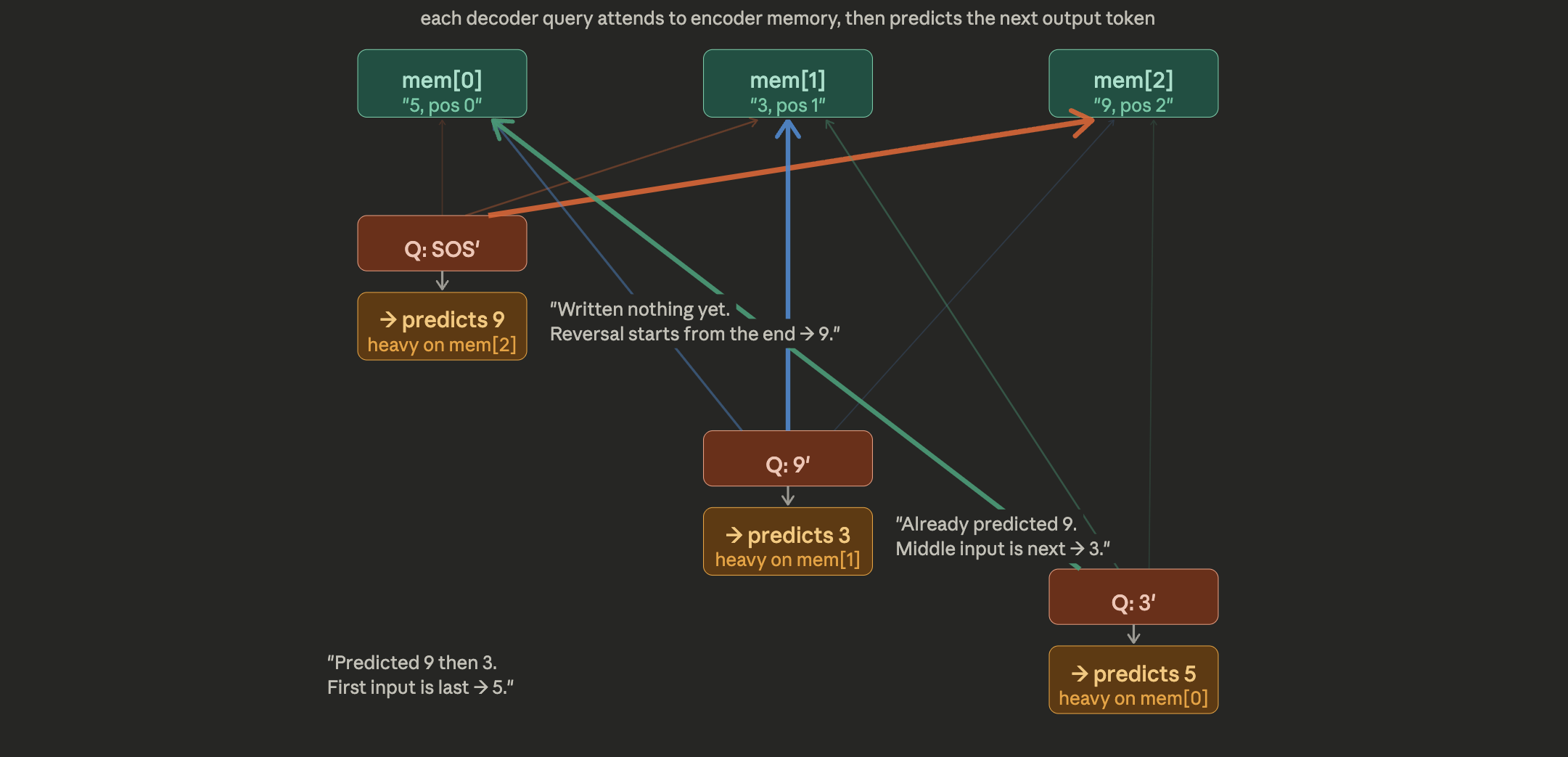
Note : It’s not exactly as predicting 9/3/5. It’s learning a representation to predict the next token using the encoder memory and previously generated tokens.

Step 6 : Feed Forward and Output layer

Just like in the encoder, after the two attention stages have done all the “token mixing,” the FFN processes each vector independently. It’s the “digest what I just learned” step — it takes the rich blend of output history (from masked self-attention) and encoder context (from cross-attention) and transforms it into a sharper, more decisive representation. Then the linear layer maps that 64-dim vector to 20 numbers — one score per vocab token. Argmax picks the winner. From the SOS position you get 9, from 9 you get 3, from 3 you get 5.

Closing Note

Transformers may look complex at first, but at their core, they follow a simple idea: represent words as vectors, add positional information, and allow each word to interact with every other word using attention.

Residual connections help preserve and refine information, while layer normalization keeps the training stable. Multi-head attention extends this idea by letting the model look at the same sentence from multiple perspectives.

Together, these components enable Transformers to build rich, context-aware representations of language without relying on sequential processing.